Modelling COVID-19 in Canada at a Provincial Level
2021-06-05
1 Introduction
This paper documents a model of the COVID-19 epidemic in Canada. Mobility data is used to model the reproduction number of the COVID-19 epidemic over time using a Bayesian hierarchical model. This is achieved by adapting the work by Imperial College London researchers [1] for Canada. Authors from Imperial College London have built similar models for Brazil [2] and the United States [3]. In this case the model is calibrated to reported COVID-19 deaths as compiled in [4].
The model uses mobility movement indexes by province produced by Google [5]. Furthermore the model includes an effect for mandatory indoor mask-wearing based on data as compiled in [6] (and extended).
The model and report are automatically generated on a regular basis using R [7]. This version contains data available on 31 May 2021.
An online, regularly updated version of this report is available here.
2 Updates
As this paper is updated over time this section will summarise significant changes. The code producing this paper is tracked using git. The git commit hash for this project at the time of generating this paper was 0be6ff42b0fdf07ed168c2ac29d13d34a3c14609 and this change was made on 2021-06-02.
2020-11-01
- First draft Canadian report.
2021-01-01
- Correct initial R plots.
- Corrected parameter estimate plots. These charts were incorrectly adding country wide effects and provincial effects.
2021-01-24
- Various updates to the report to bring in line with changes made in SA report.
- Adding additional results on 30 June 2021.
- Add worst case projection.
2021-04-29
- Update projection dates to 30 June and 30 September 2021.
2021-06-01
- Adjust mobility scenarios.
3 Methodology
A detailed description of the methodology and assumptions is provided below below. The key features of the approach employed are summarised here:
- It uses a Bayesian Hierarchical Model to calibrate model parameters based on observed excess death data and prior assumptions.
- Changes in the reproduction number are linked to mobility data [5], mandatory indoor mask-wearing, as well as an autoregressive term.
- The reproduction number over time is used to model the number of infections occurring over time.
- The model uses population-weighted infection fatality ratios (IFRs) by province with some noise added as well as assumptions about the time it takes to die to model deaths from infections.
- There is a single combined model for all provinces. This model shares information between provinces, but province-specific effects are also allowed.
- Provinces with less data have been grouped together.
- The model is fitted such that it uses the prior assumptions about various parameters as well as the reported death data in such a way to provide an updated parameter distribution and outcome distribution that reflect both the prior assumptions as well as the reported COVID-19 death data.
4 Mobility
4.1 National Mobility Data
The national mobility data from [5] is plotted below. The model uses the indexes at a provincial level but here the national indexes are plotted for convenience. Clear trends are observable.
- Mobility generally reduces from late March
- Residential mobility increases from late March.
- Park related mobility increases over the summer months.
- Other mobility generally increases after the initial decrease in March.
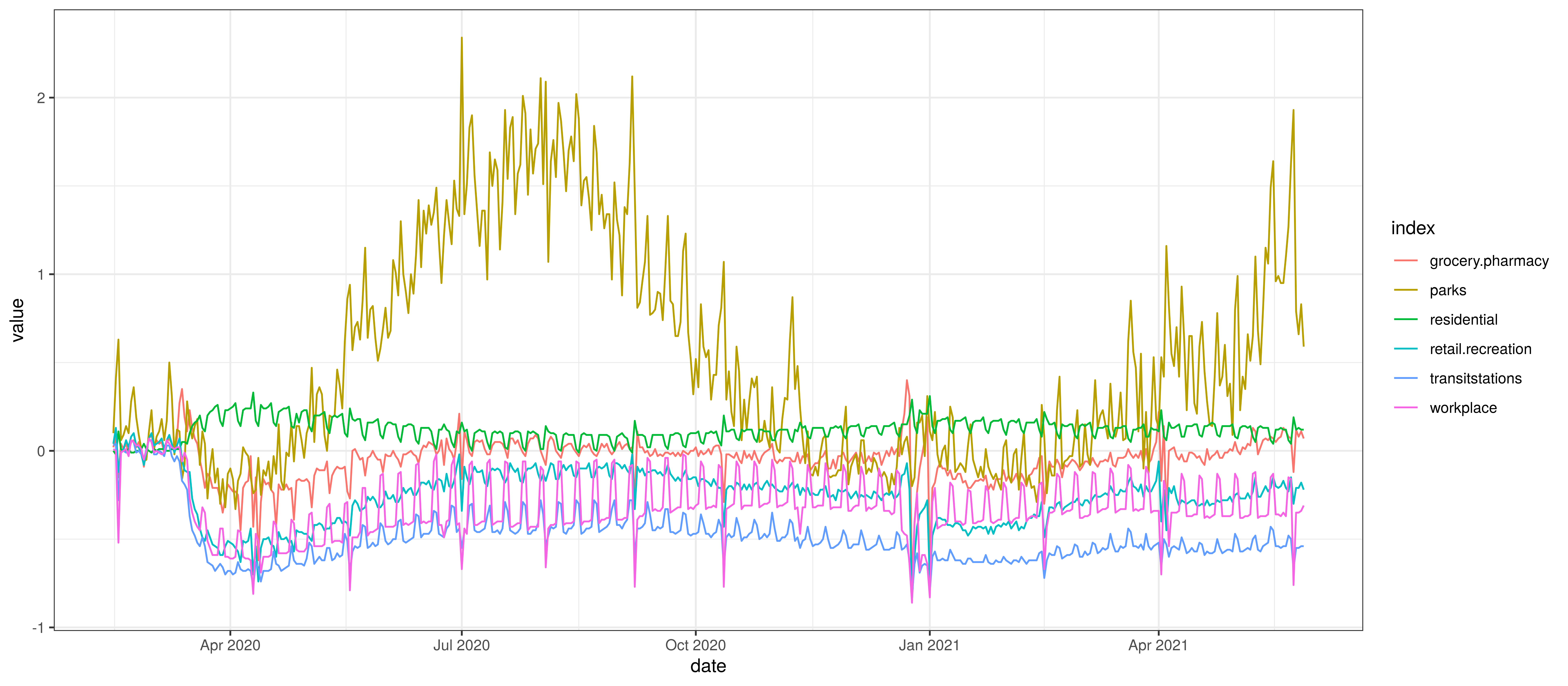
Google Mobility Indexes for Canada
The chart below summarises the average mobility index used in the model. This is the average of mobility indicators excluding parks and residential. This follows [8].
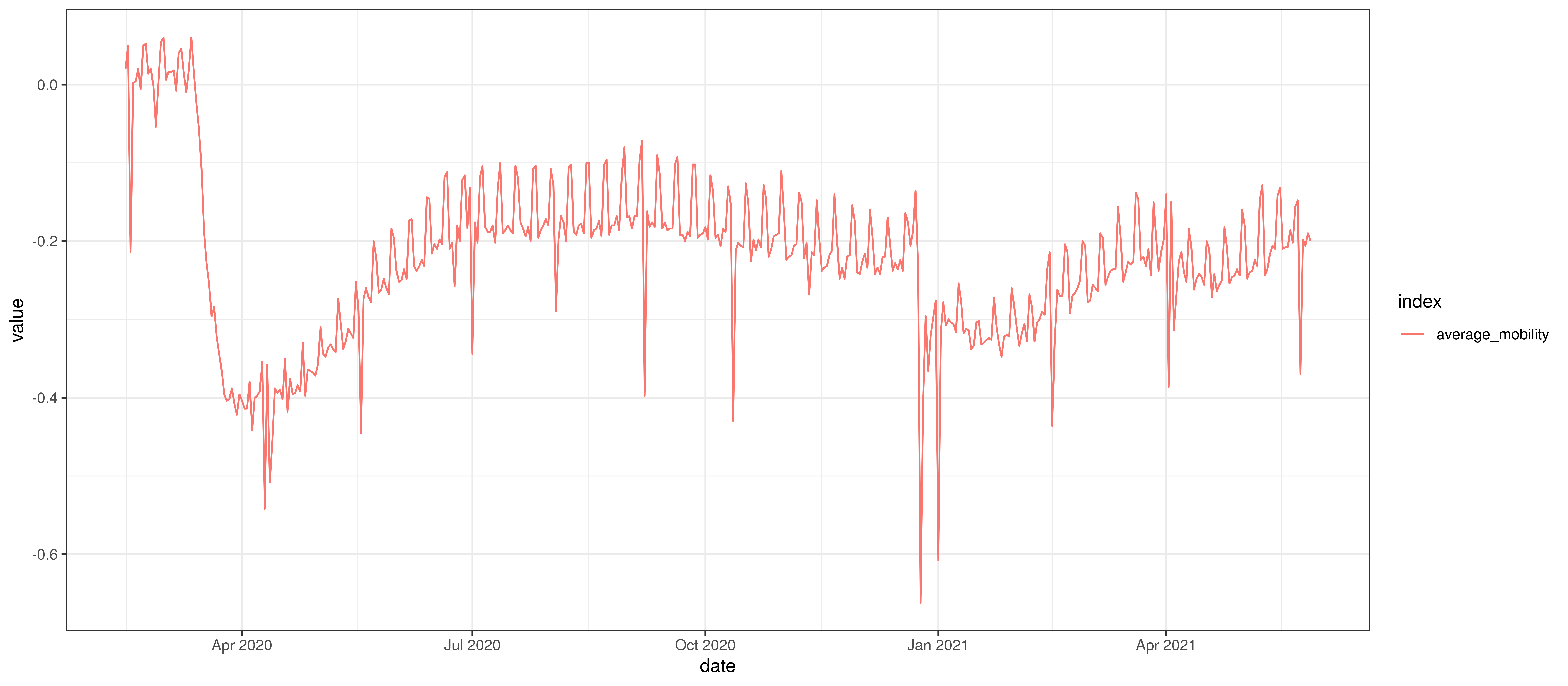
Average Mobility
4.2 Provincial Mobility Data
The average mobility (excluding residential & park indexes) is plotted below for the various provinces. Grouped provinces uses mobility weighted by the population of provinces where there is mobility data available.
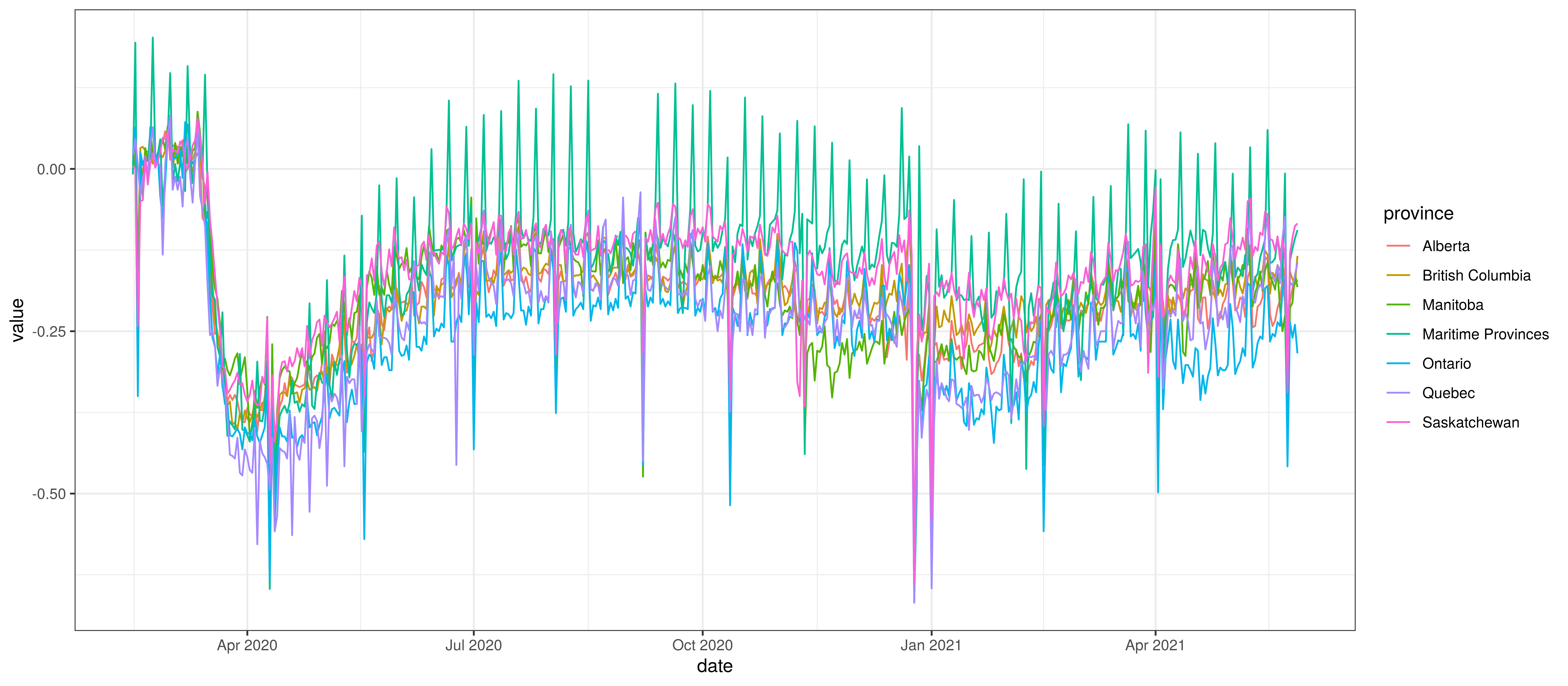
Average Mobility by Province
5 Mandatory Indoor Mask-Wearing
Mandatory mask-wearing mandates are compiled by province in [6]. This data contains a single indicator by province with 0 indicating no mandate and 1 indicating a province wide mandate. The authors also used numbers between 0 and 1 to indicate mandates that affected only subsets of the population.
The grouped provinces use a weighted average (by population) of the mask-wearing indicator from the respective provinces.
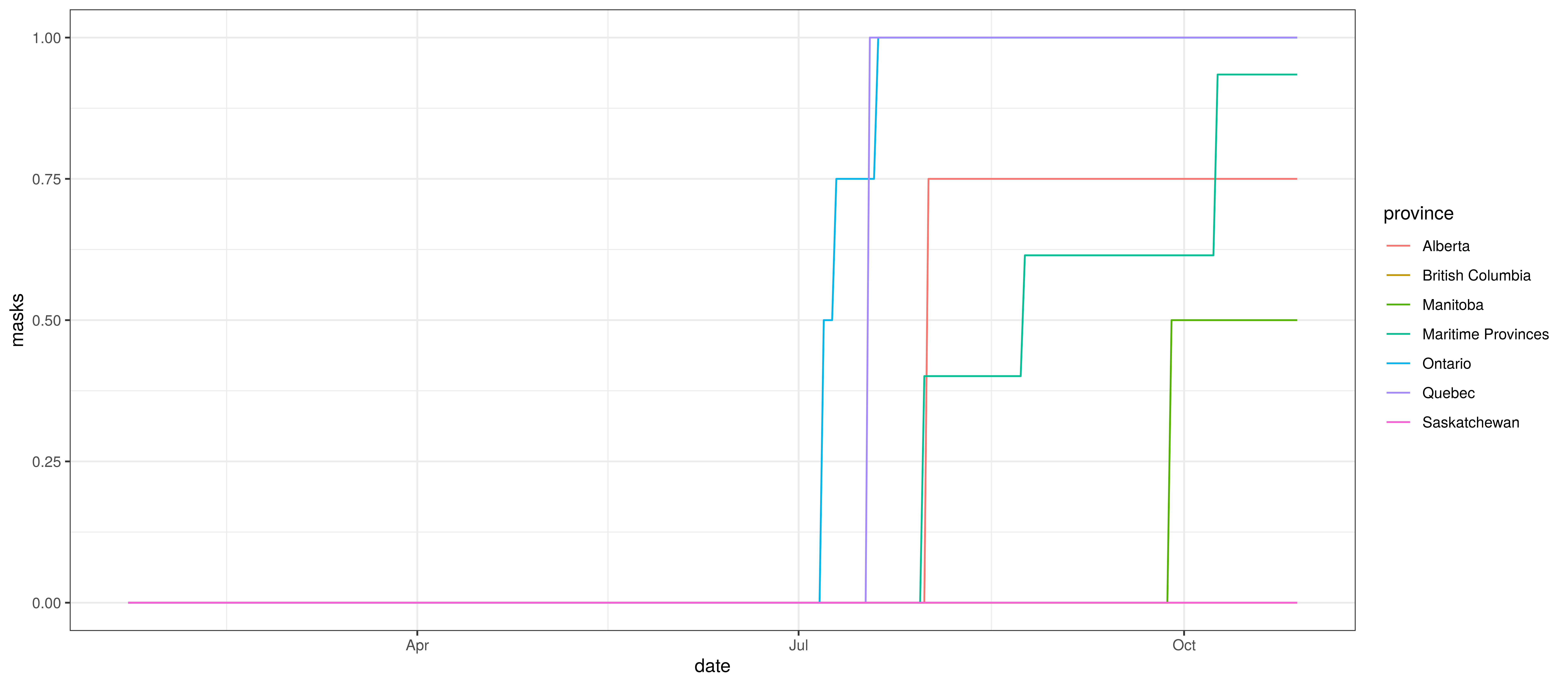
Mandatory Indoor Mask-Wearing by Province
6 Calibration
The sections below show how well the model is reproducing past data. Various panels are plotted for each province:
- The first shows the daily count of deaths reported in the province (brown) and the estimated deaths in blue. This shows how well the model is calibrated to reported deaths.
- The second panel shows the modelled daily number of infections (blue) compared to confirmed case counts (brown) as reported for the province. Note that this model does not calibrate to case data, but this data is shown for reference. It is expected that the model would produce infections exceeding confirmed cases as testing is likely only finding a fraction of the true infections.
- The third panel shows the estimates for reproduction number (\(R_{t,m}\)) over time (\(t\)) for each province (\(m\)). These values are generating the infections in the model which result in deaths. Note that due to the delay of deaths following infections the last week or two of \(R_{t,m}\) values already present an extrapolation from the data. Deaths as a result of these recent infections have generally not occurred as yet.
- The final panel shows the estimated value of \(2\cdot\phi^{-1}(-\epsilon_{w_m(t),m}))\). This unexplained value converted to a factor of \(R_{t,m}\). A value greater than 1 indicates that the \(R_{t,m}\) was higher than the value implied by other parameters. A value below 1 indicates the reverse.
In all the charts the darker shaded area represents a confidence interval of 50% and the lighter shaded area represents a confidence interval of 95%.
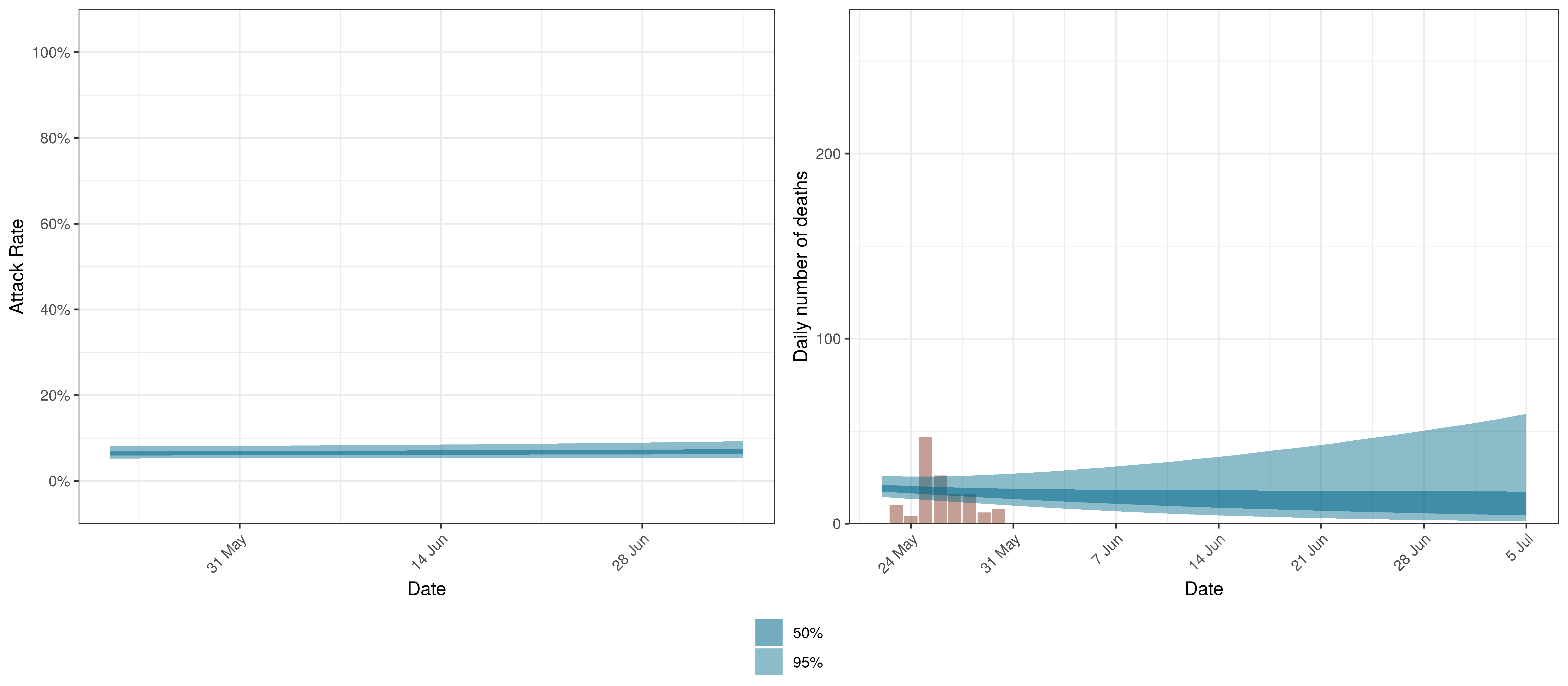
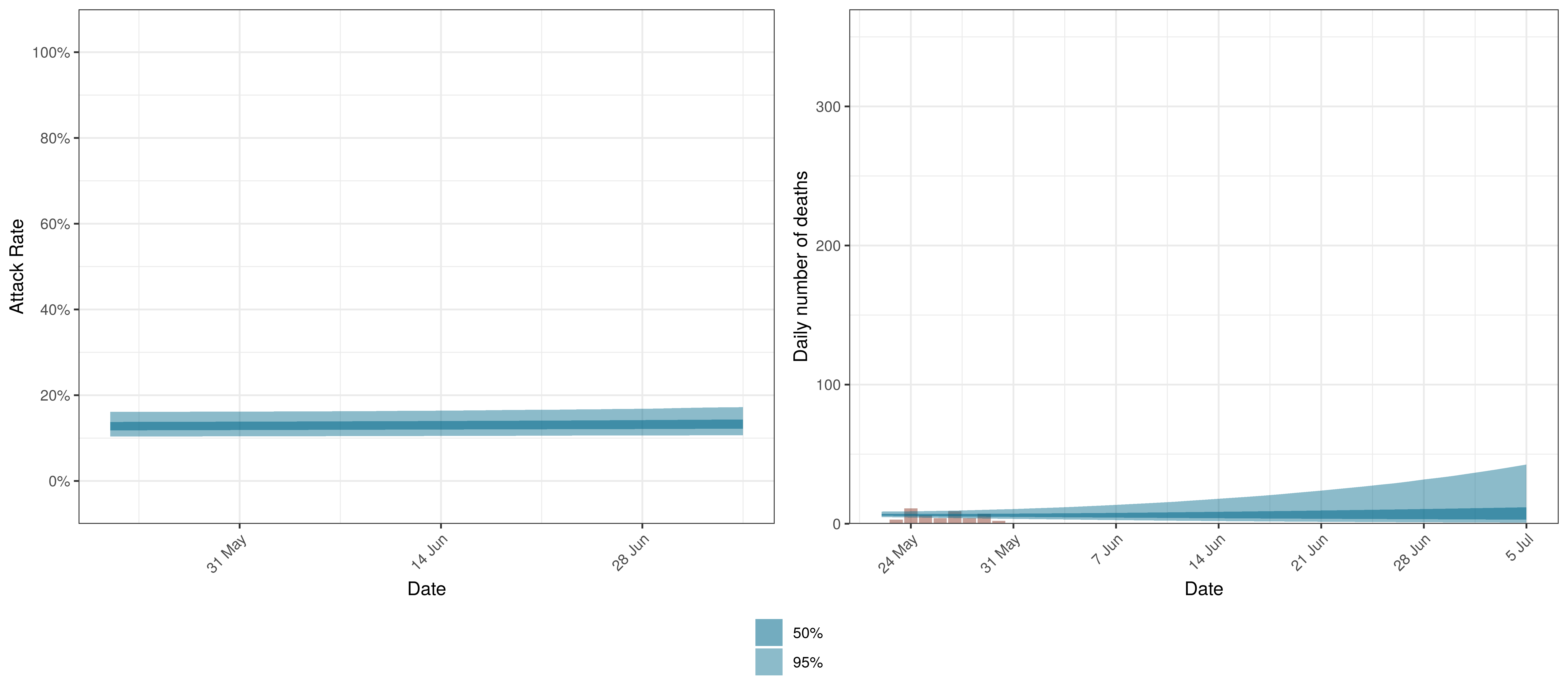
6.1 Alberta
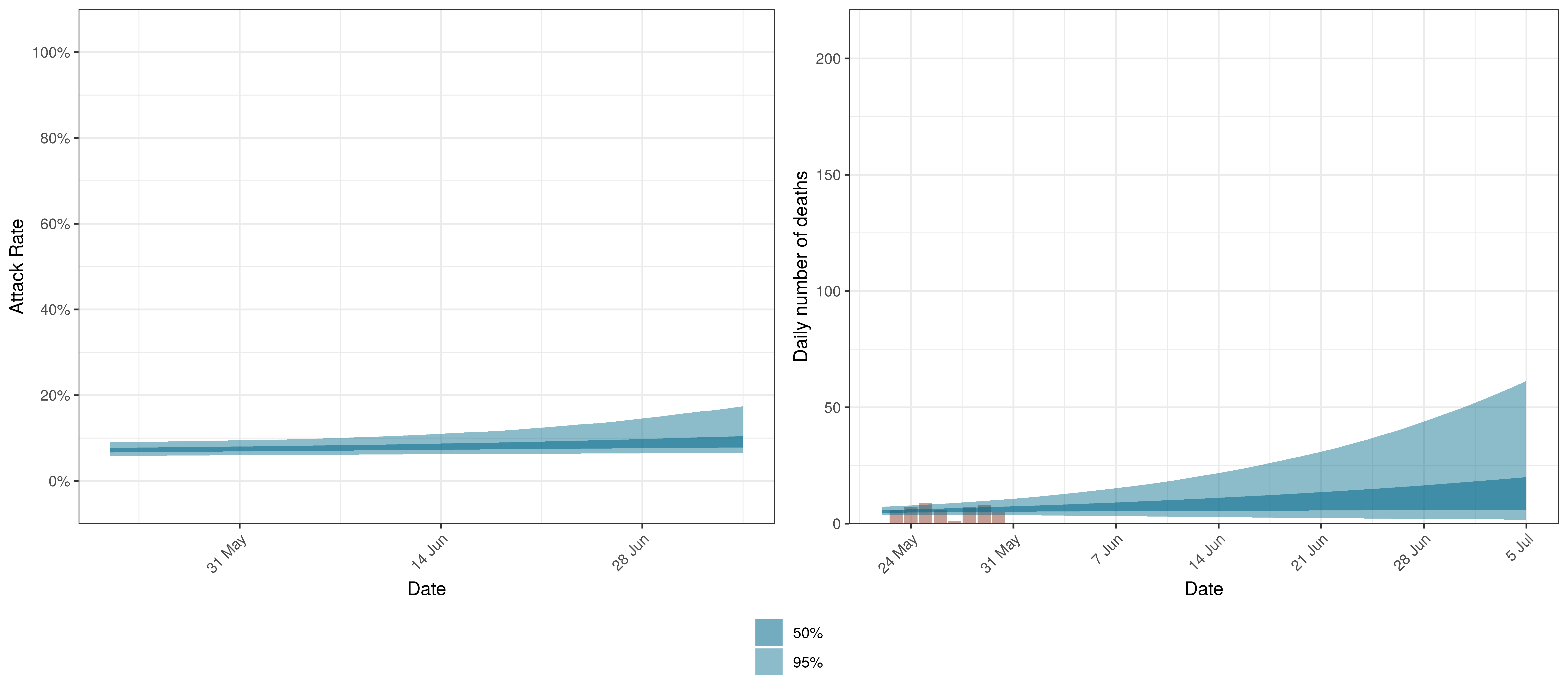
The reported deaths (in brown) and estimated deaths (in blue) are plotted below. The calibration appears reasonable.
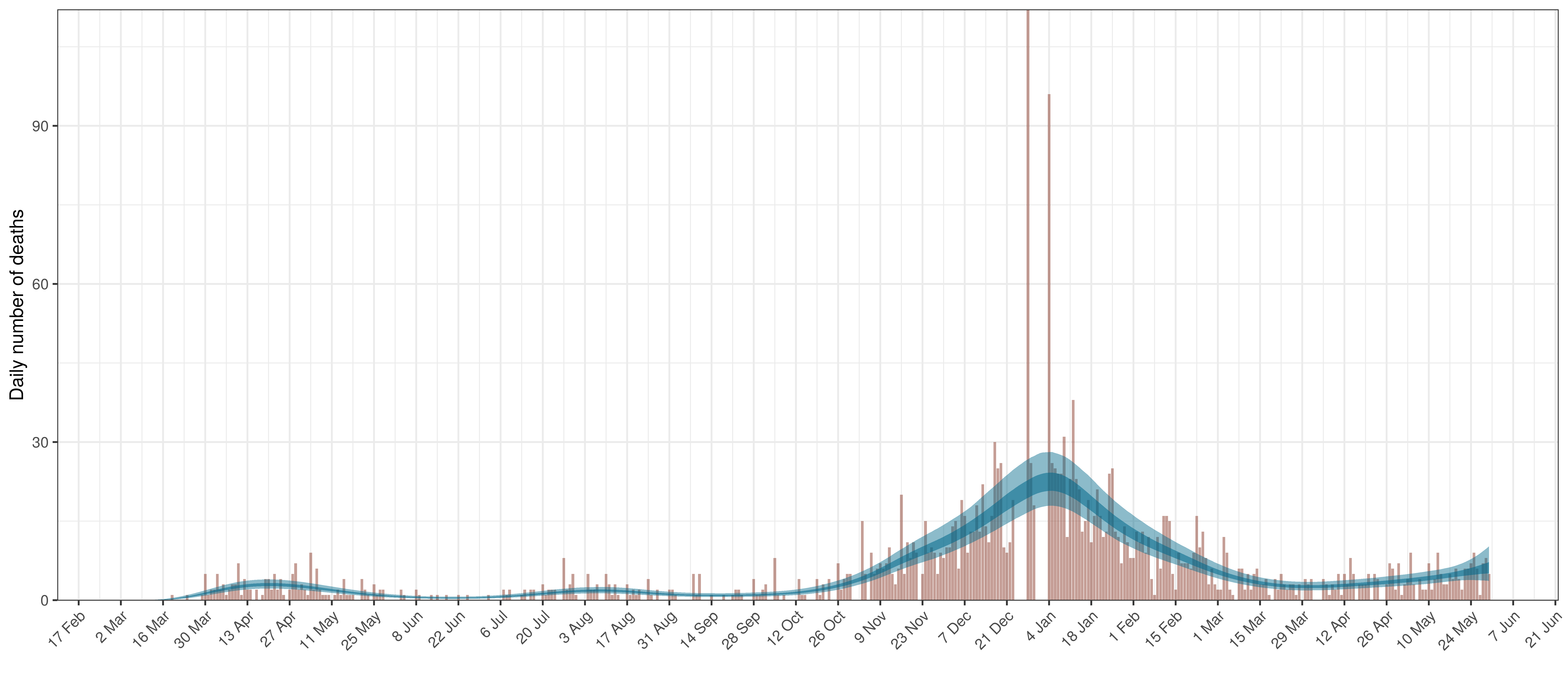
Projected Deaths compared to Reported COVID-19 Deaths in Alberta
Below modelled infections are plotted compared to confirmed cases. Over the last 14 days it would appear that 47.8% of all new infections were tested.
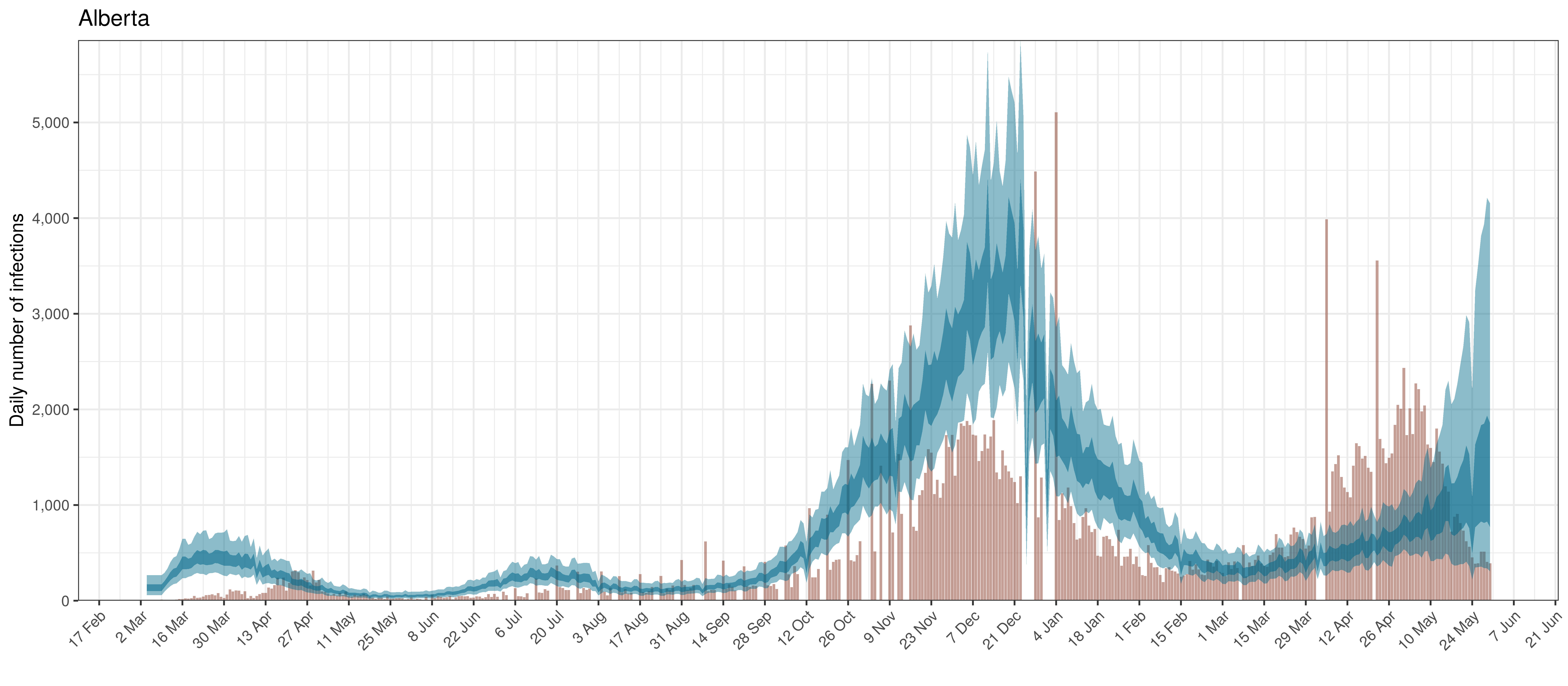
Projected Infections compared to Confirmed Cases in Alberta
Below the \(R_{t,m}\) is plotted.
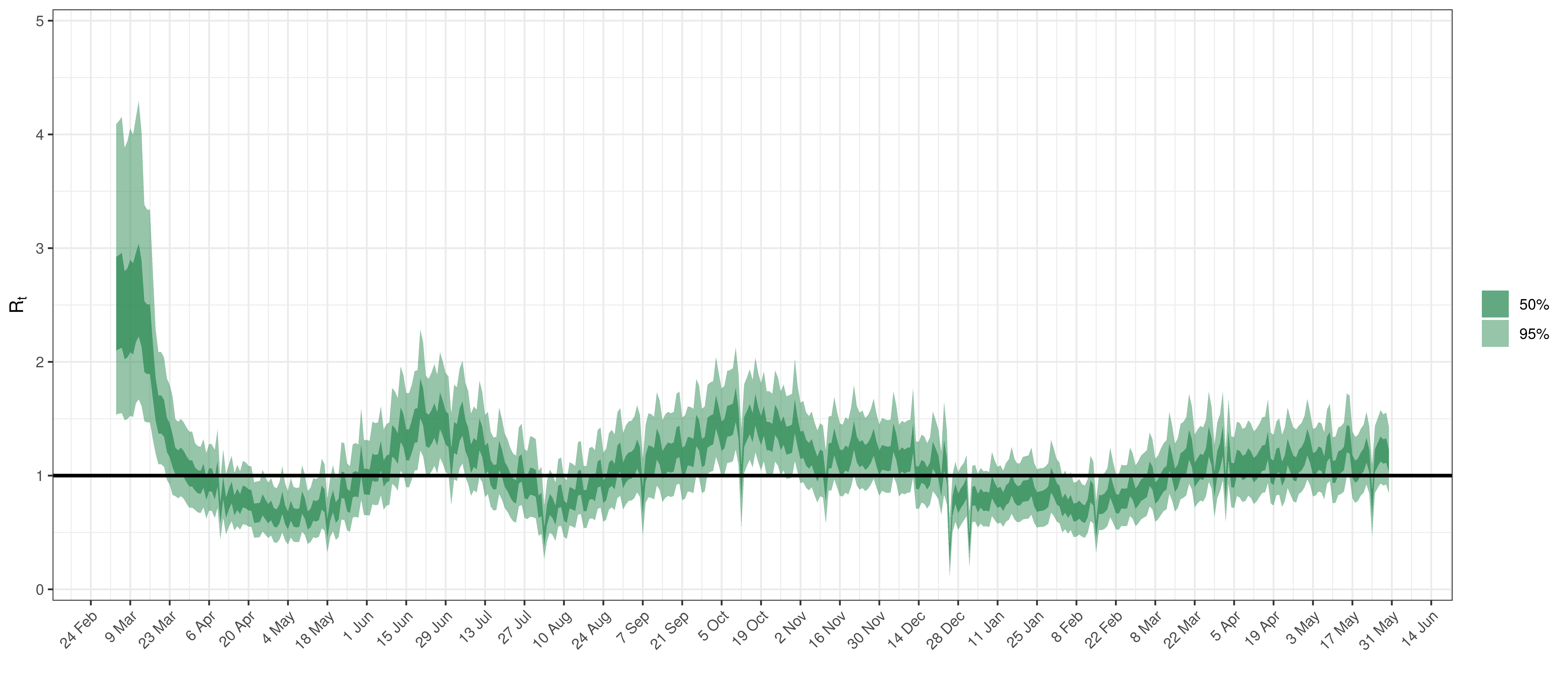
Effective Reproduction Number in Alberta
Below the \(2\cdot\phi^{-1}(-\epsilon_{w_m(t),m}))\) is plotted.
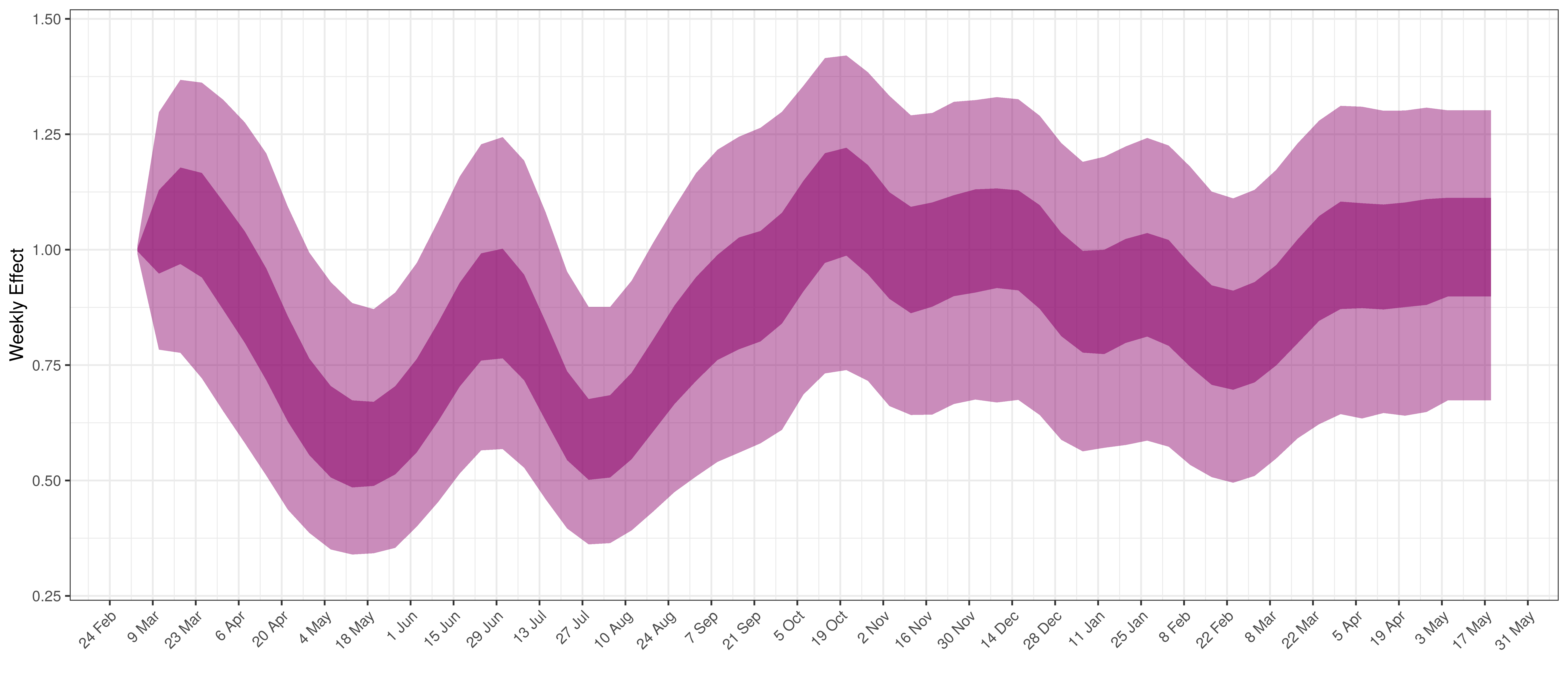
Weekly AR(2) Factor Plot for Alberta
6.2 British Columbia
The reported deaths (in brown) and estimated deaths (in blue) are plotted below. The calibration appears reasonable.
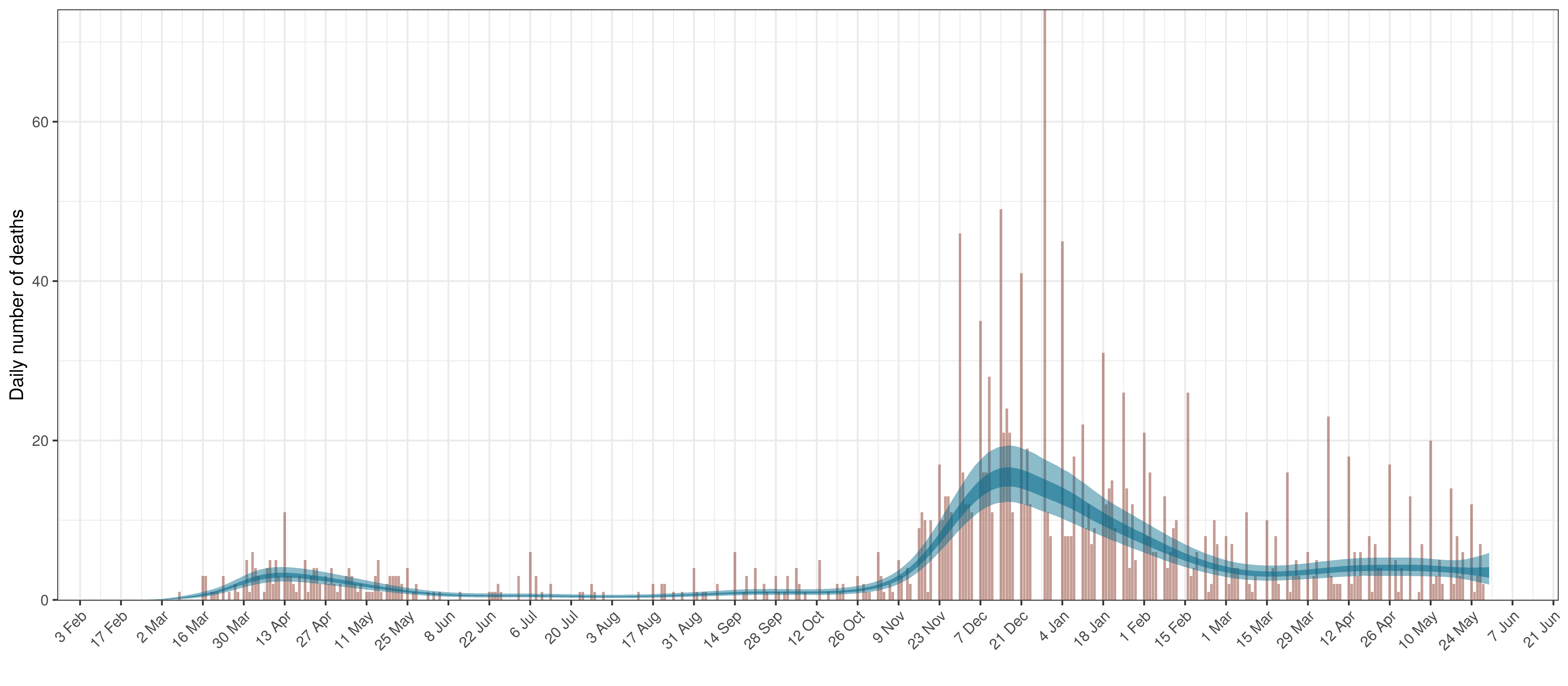
Projected Deaths compared to Reported COVID-19 Deaths in British Columbia
Below modelled infections are plotted compared to confirmed cases. Over the last 14 days it would appear that 112.8% of all new infections were tested.
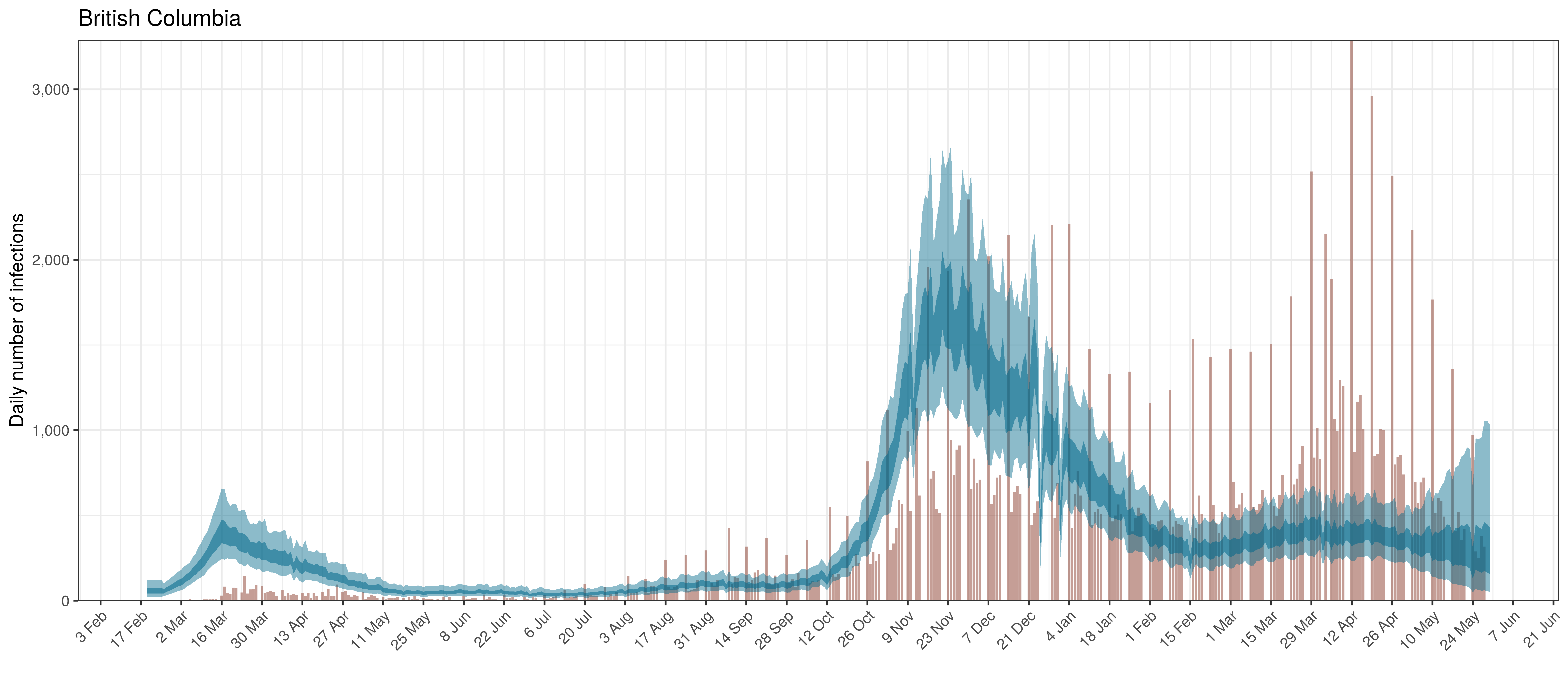
Projected Infections compared to Confirmed Cases in British Columbia
Below the \(R_{t,m}\) is plotted.
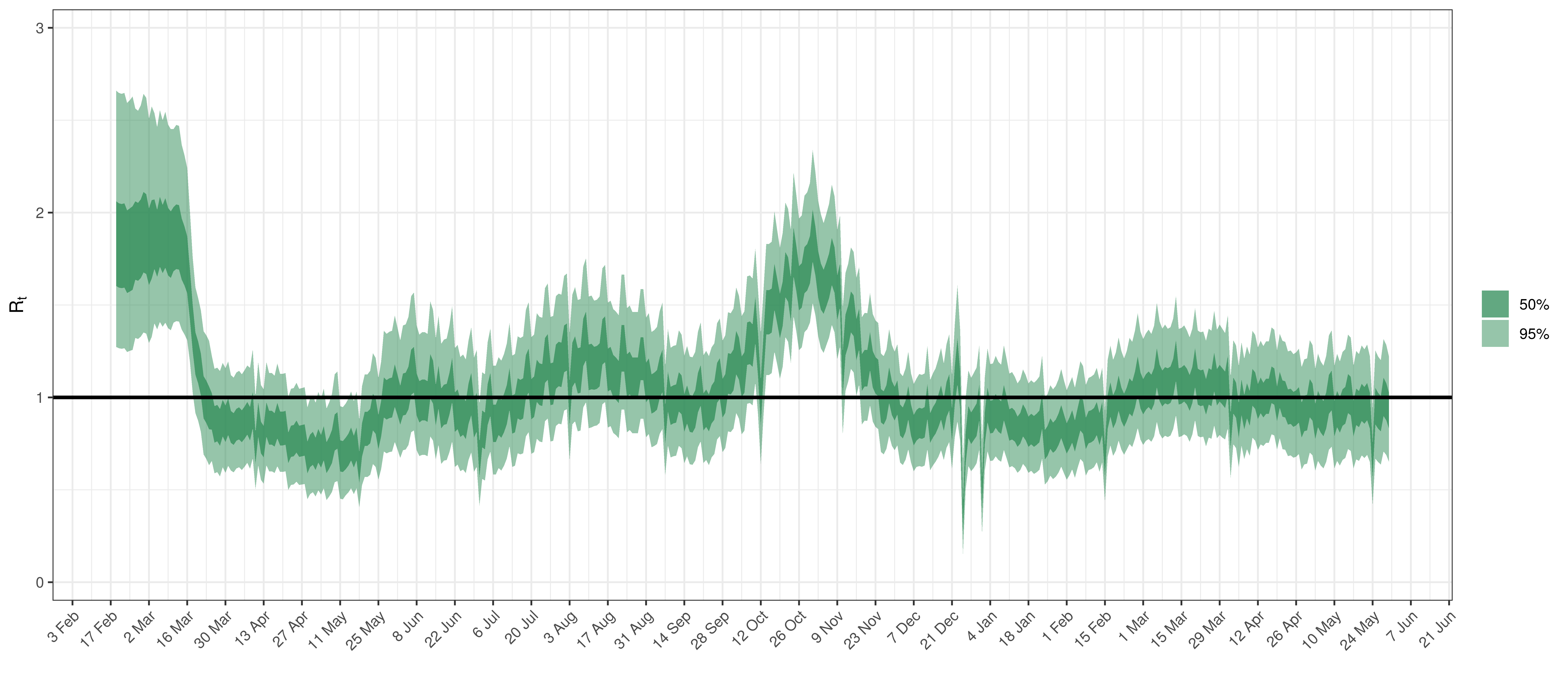
Effective Reproduction Number in British Columbia
Below the \(2\cdot\phi^{-1}(-\epsilon_{w_m(t),m}))\) is plotted.
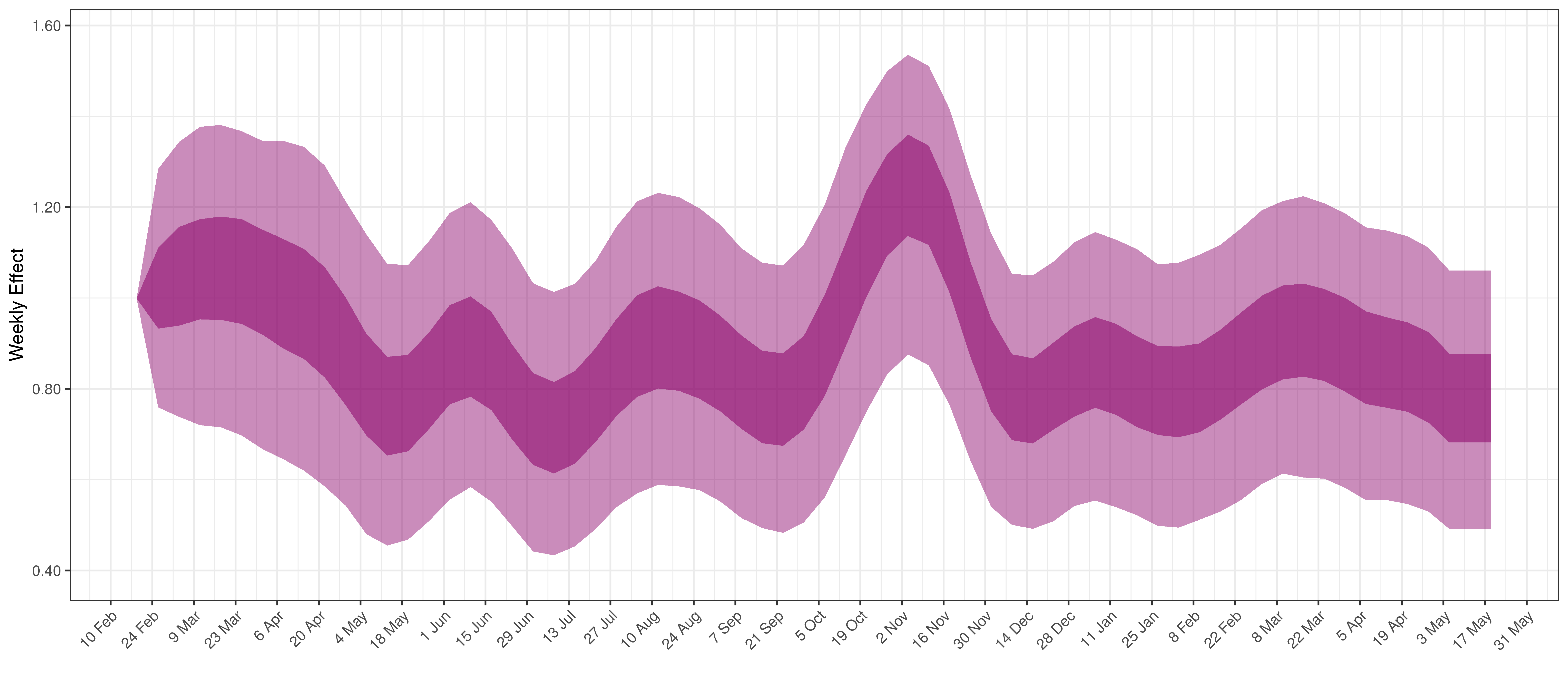
Weekly AR(2) Factor Plot for British Columbia
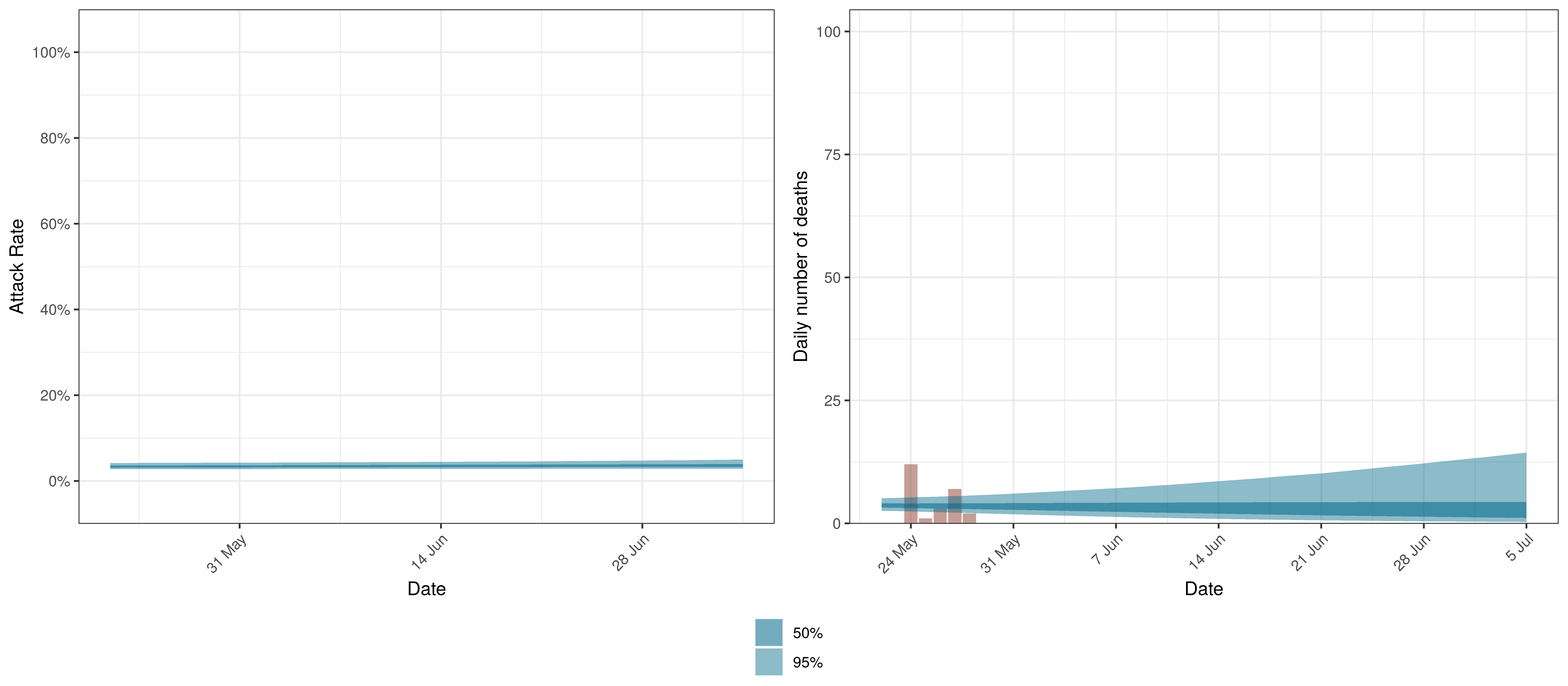
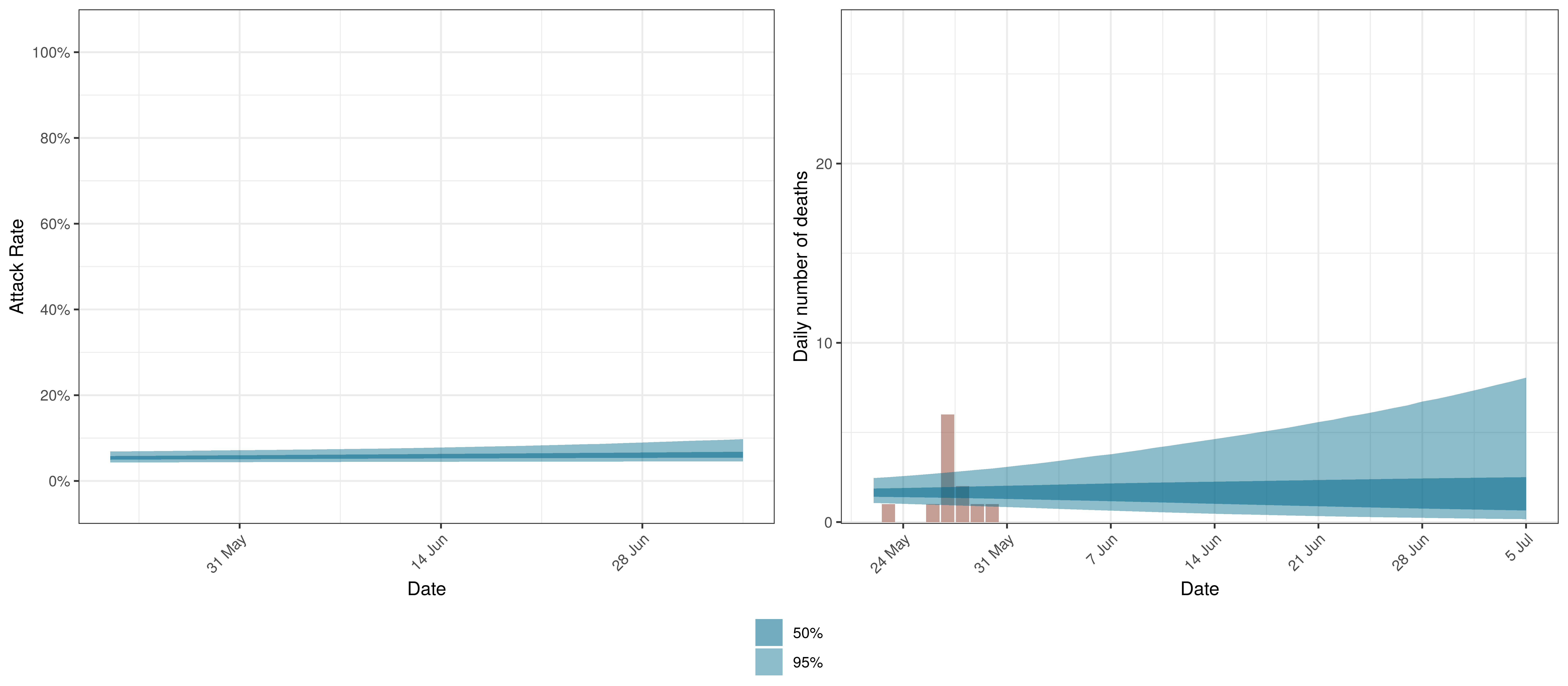
6.3 Manitoba
The reported deaths (in brown) and estimated deaths (in blue) are plotted below. Reported deaths are still low but rising.
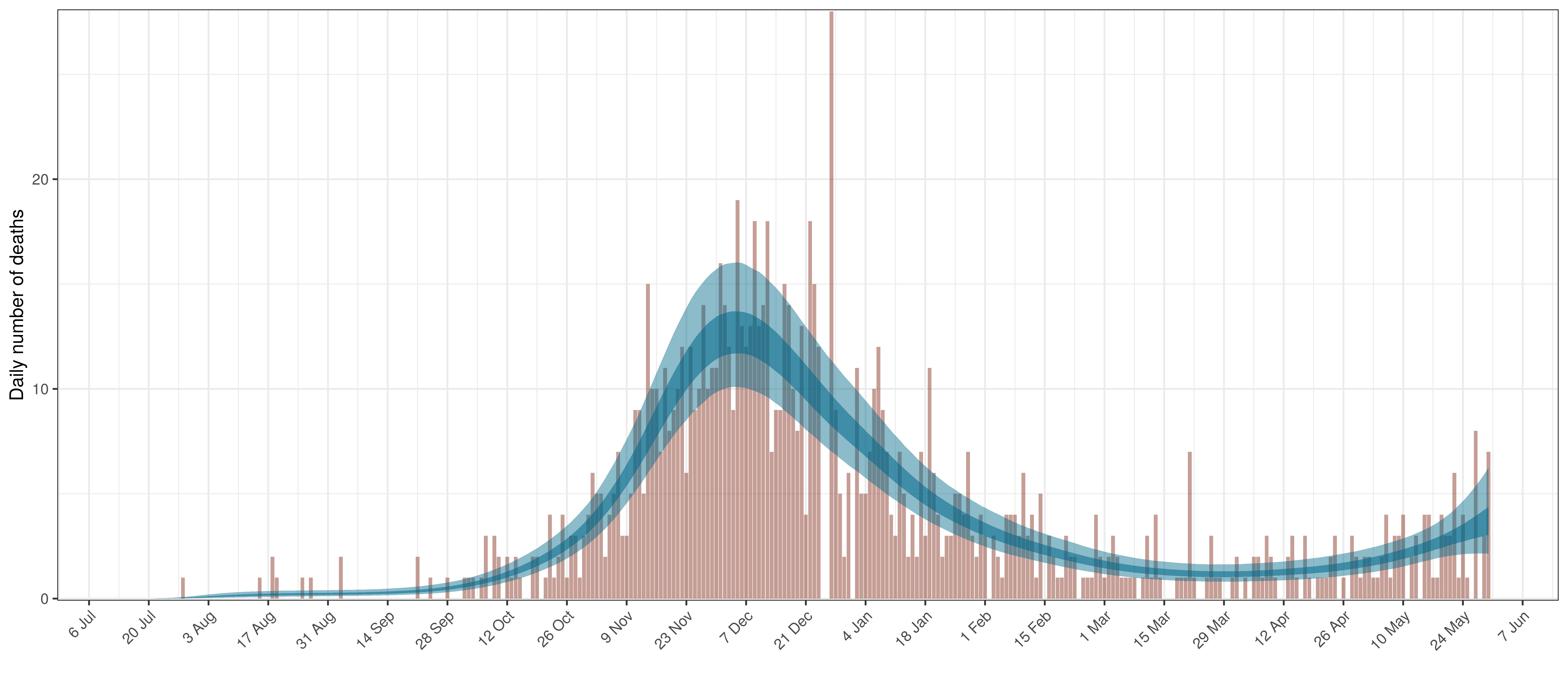
Projected Deaths compared to Reported COVID-19 Deaths in Manitoba
Below modelled infections are plotted compared to confirmed cases. Over the last 14 days it would appear that 61.9% of all new infections were tested.
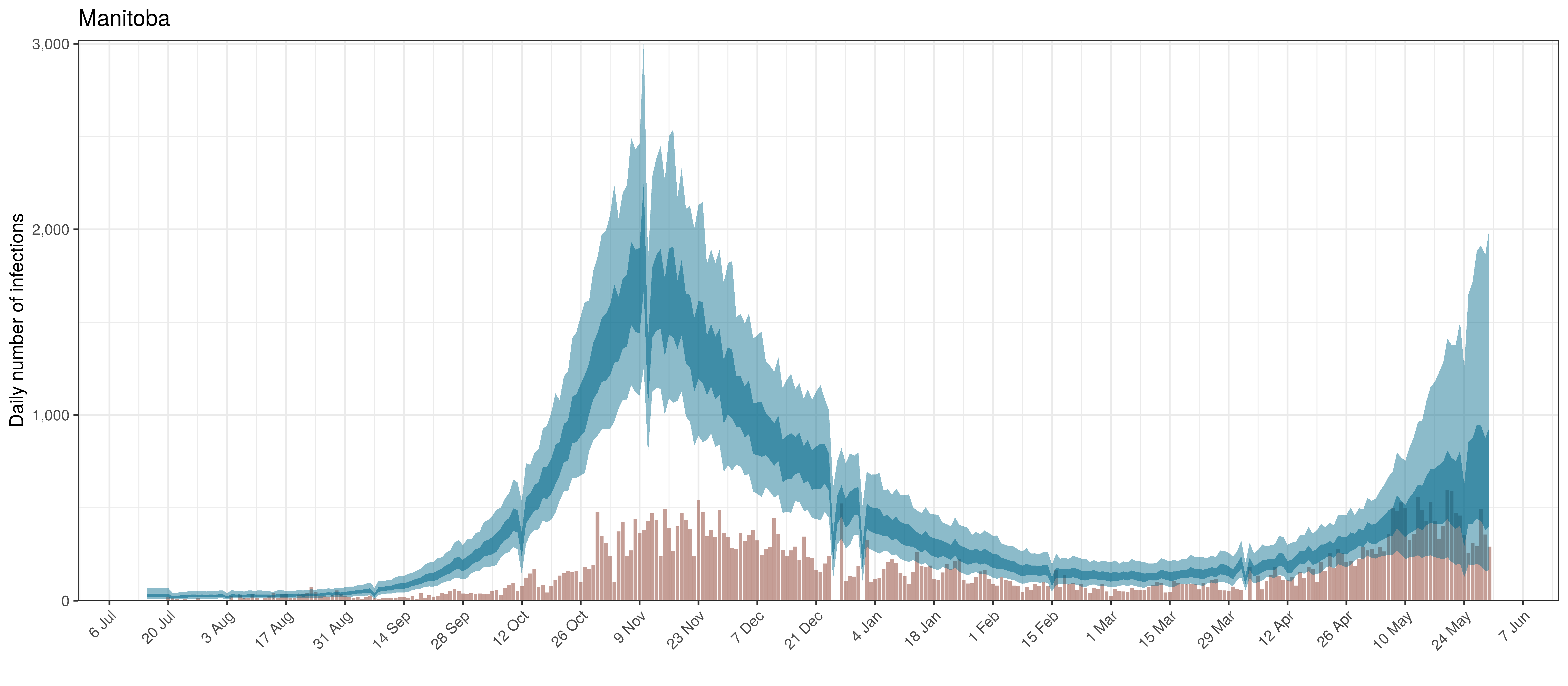
Projected Infections compared to Confirmed Cases in Manitoba
Below the \(R_{t,m}\) is plotted.
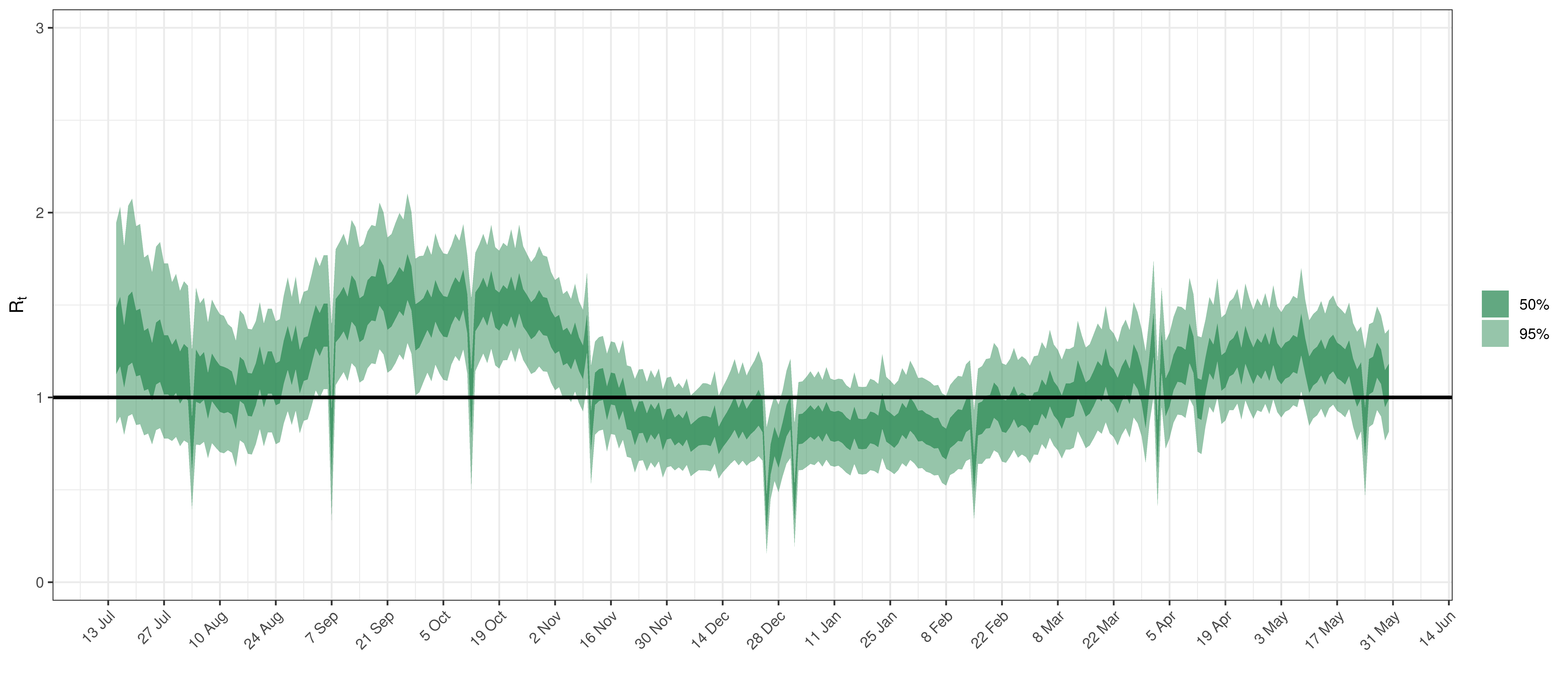
Effective Reproduction Number in Manitoba
Below the \(2\cdot\phi^{-1}(-\epsilon_{w_m(t),m}))\) is plotted.
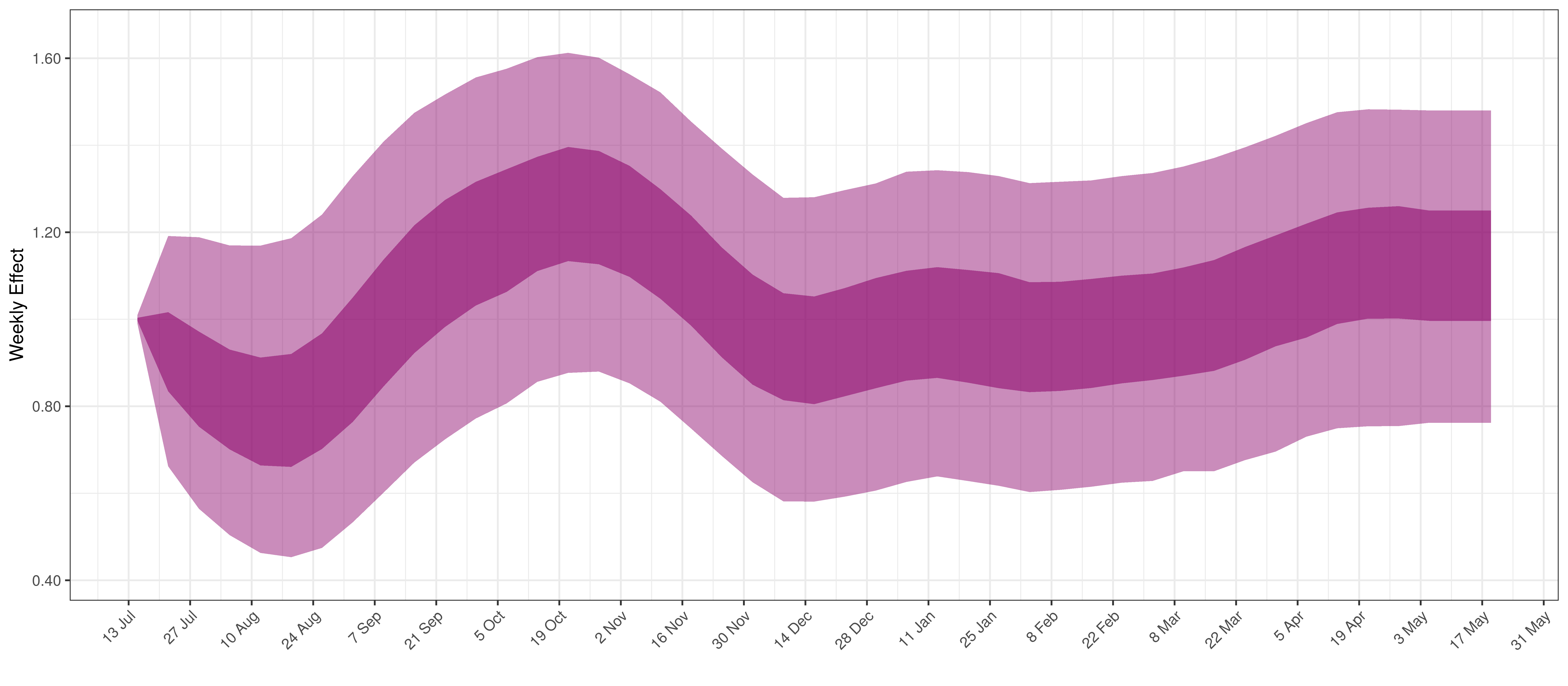
Weekly AR(2) Factor Plot for Manitoba
6.4 Maritime Provinces
The reported deaths (in brown) and estimated deaths (in blue) are plotted below. There are limited recently reported deaths.
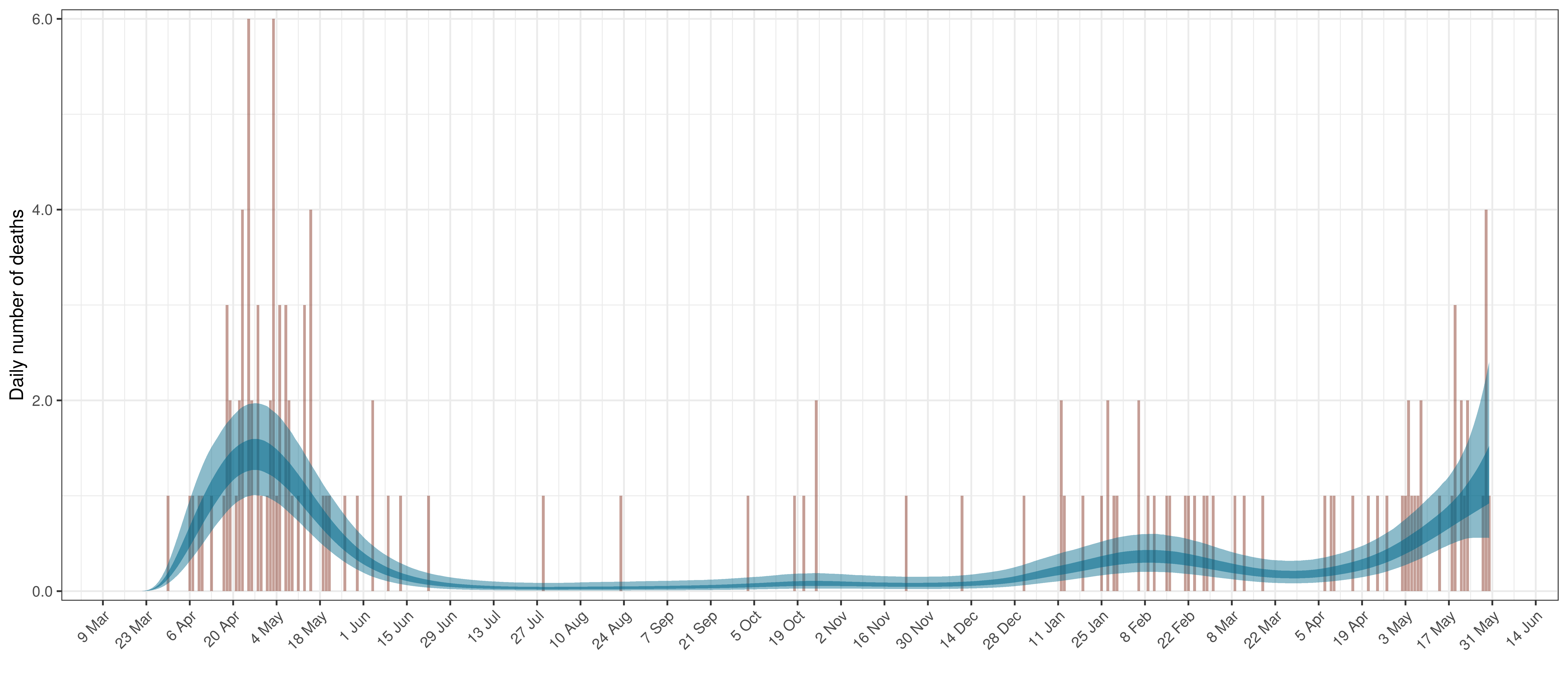
Projected Deaths compared to Reported COVID-19 Deaths in Ontario
Below modelled infections are plotted compared to confirmed cases. Over the last 14 days it would appear that 36.2% of all new infections were tested.
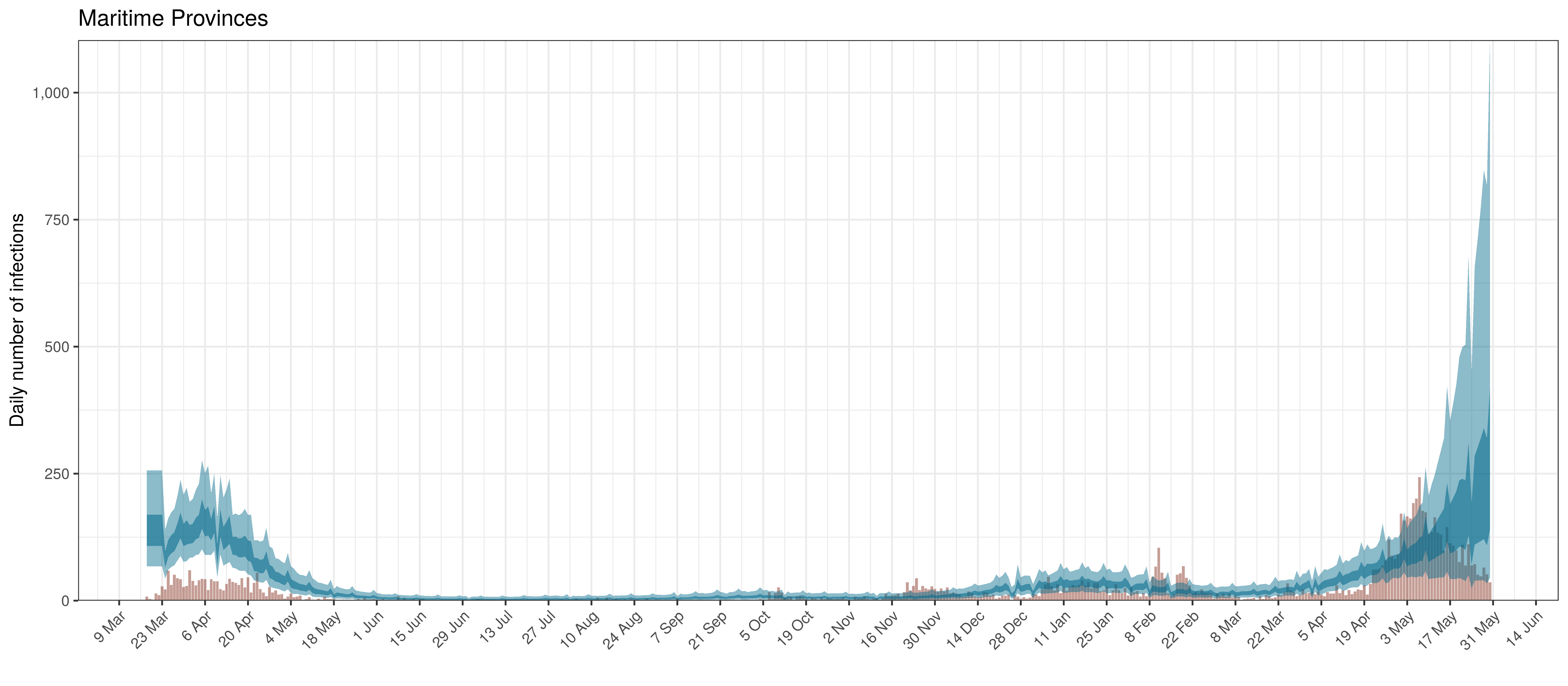
Projected Infections compared to Confirmed Cases in Maritime Provinces
Below the \(R_{t,m}\) is plotted.
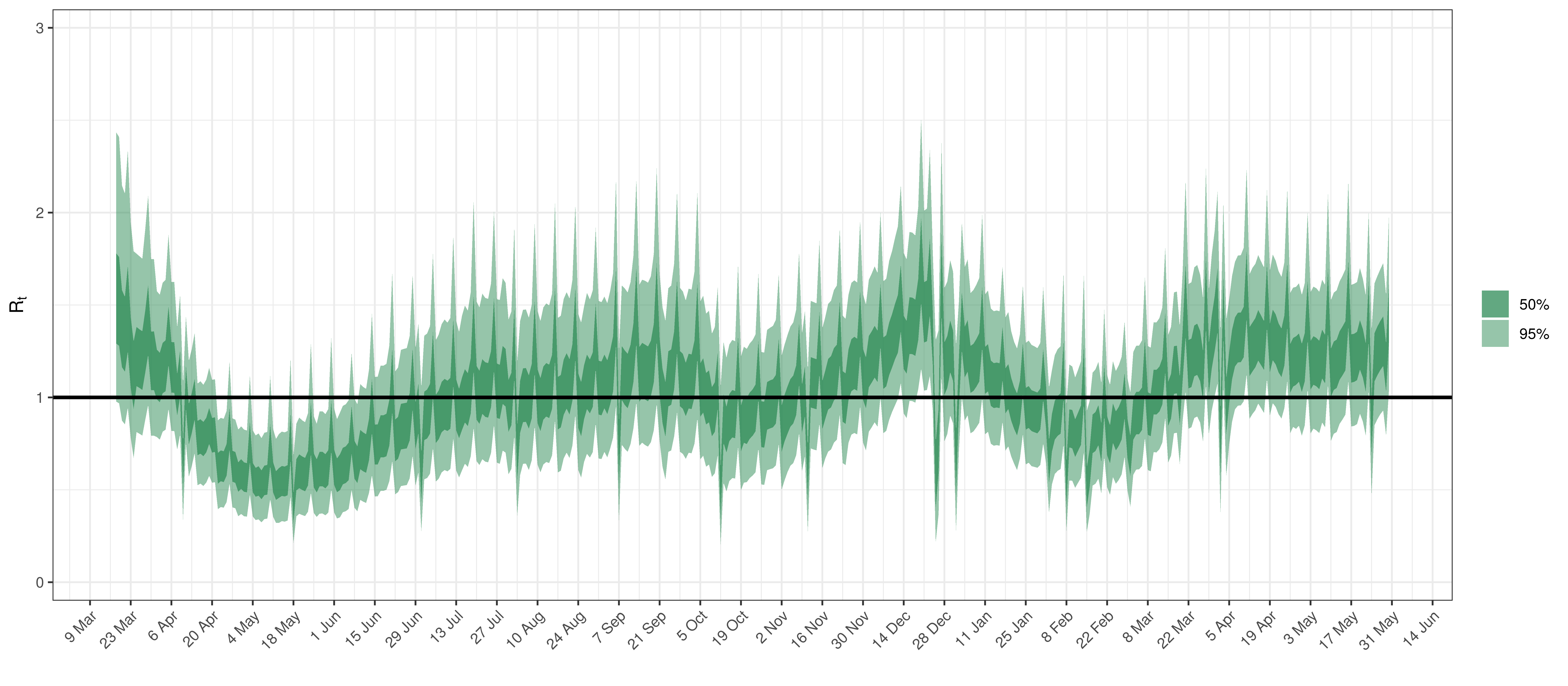
Effective Reproduction Number in Maritime Provinces
Below the \(2\cdot\phi^{-1}(-\epsilon_{w_m(t),m}))\) is plotted.
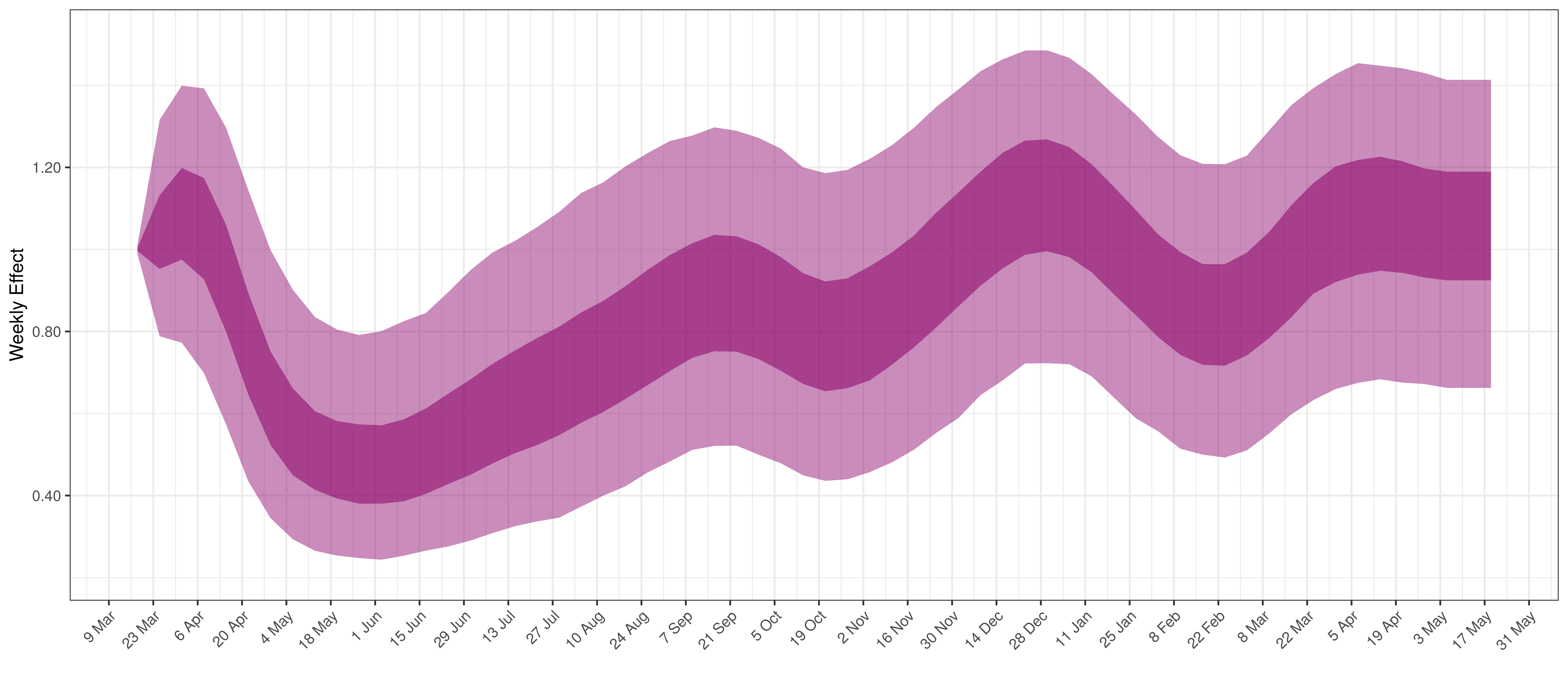
Weekly AR(2) Factor Plot for Maritime Provinces
6.5 Ontario
The reported deaths (in brown) and estimated deaths (in blue) are plotted below. The calibration appears reasonable.
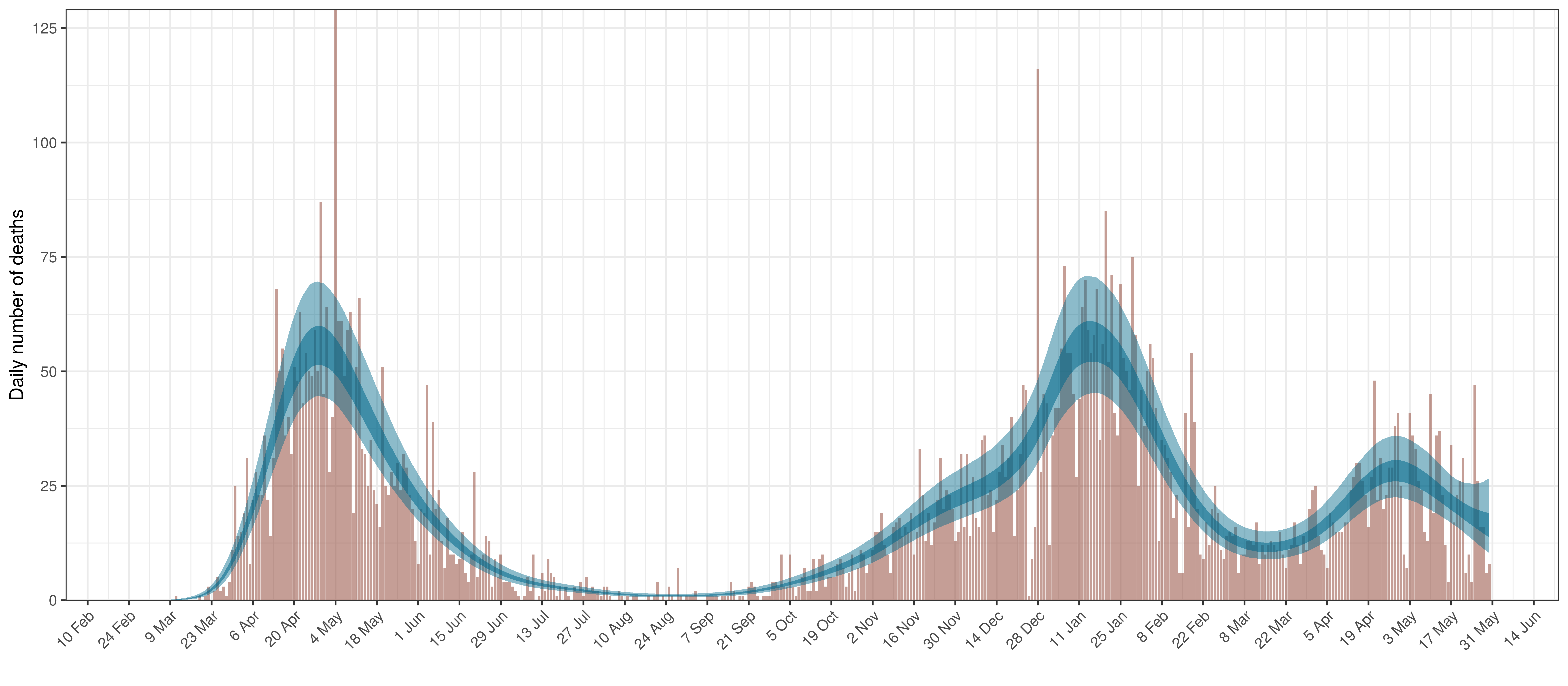
Projected Deaths compared to Reported COVID-19 Deaths in Ontario
Below modelled infections are plotted compared to confirmed cases. Over the last 14 days it would appear that 97.9% of all new infections were tested.
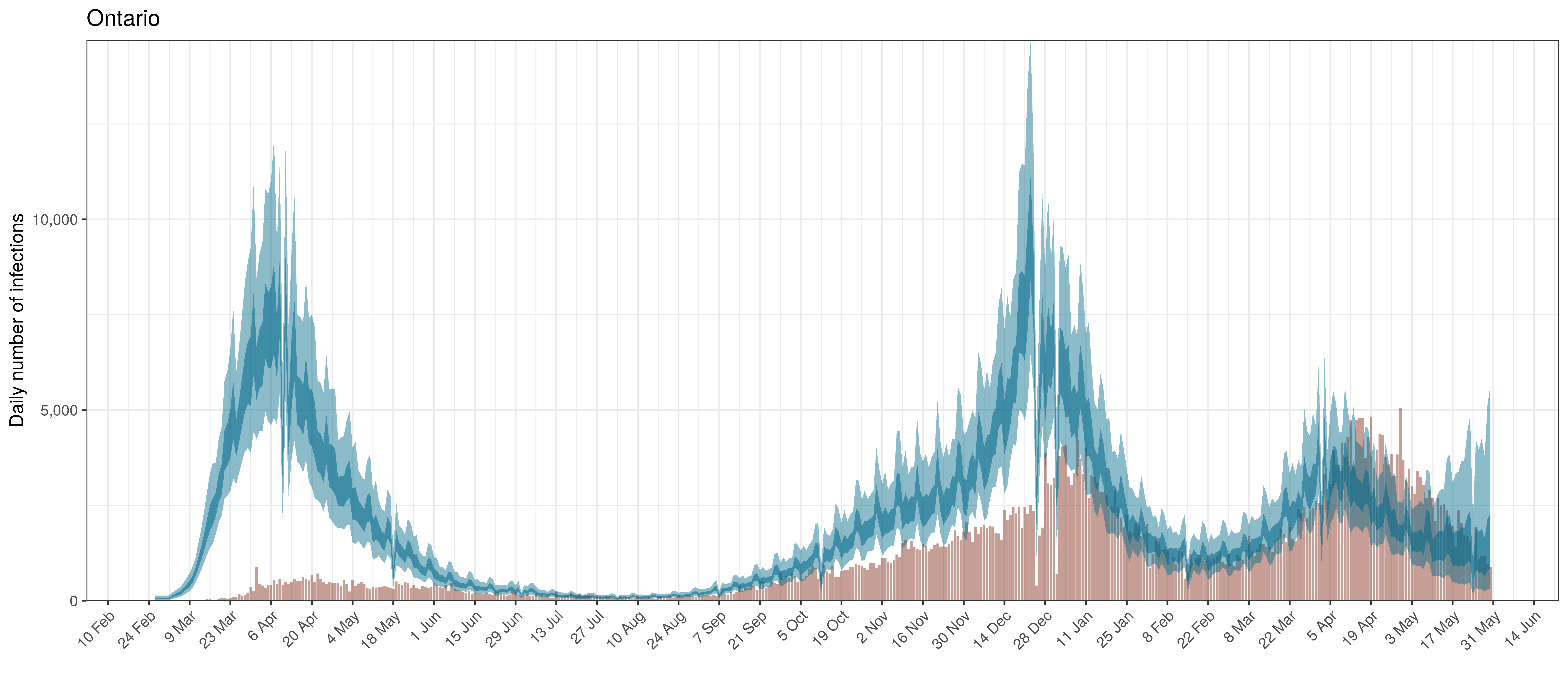
Projected Infections compared to Confirmed Cases in Ontario
Below the \(R_{t,m}\) is plotted.
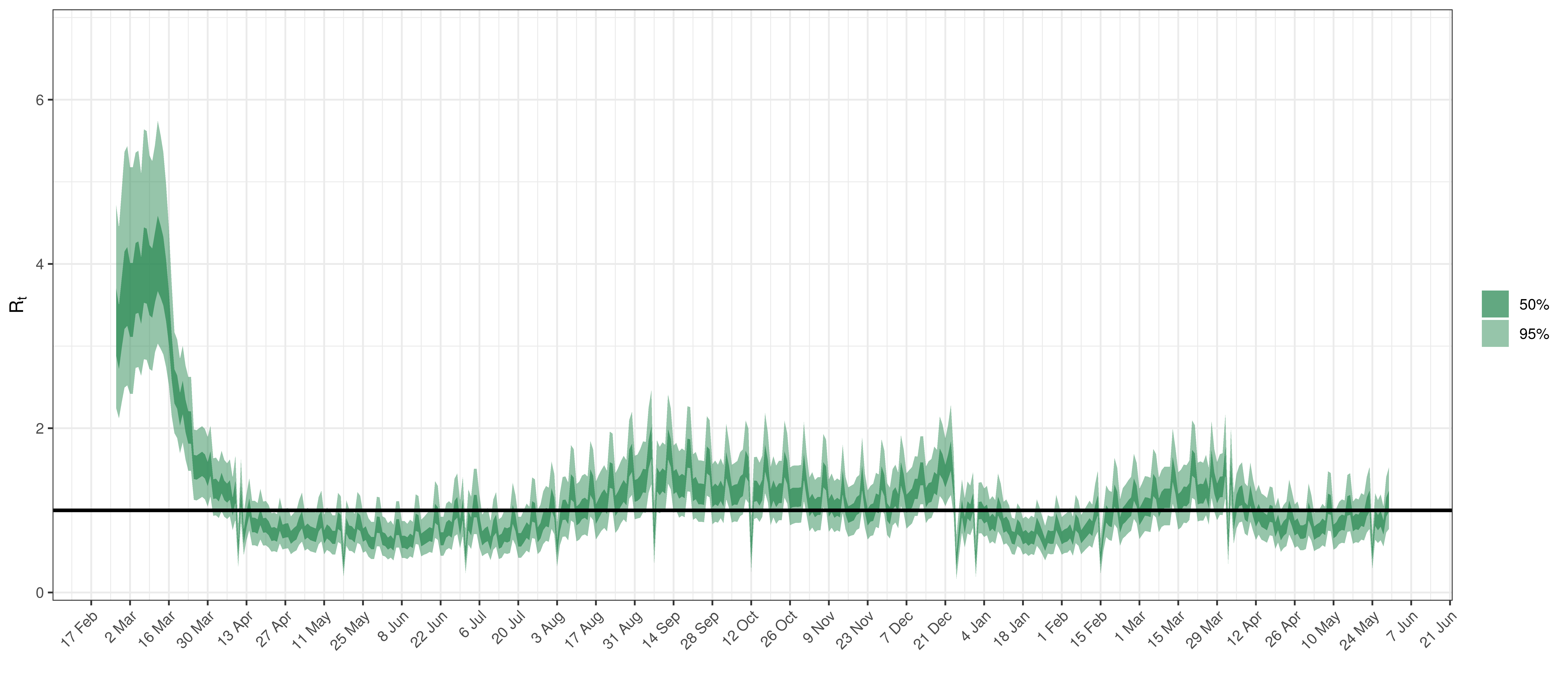
Effective Reproduction Number in Ontario
Below the \(2\cdot\phi^{-1}(-\epsilon_{w_m(t),m}))\) is plotted.
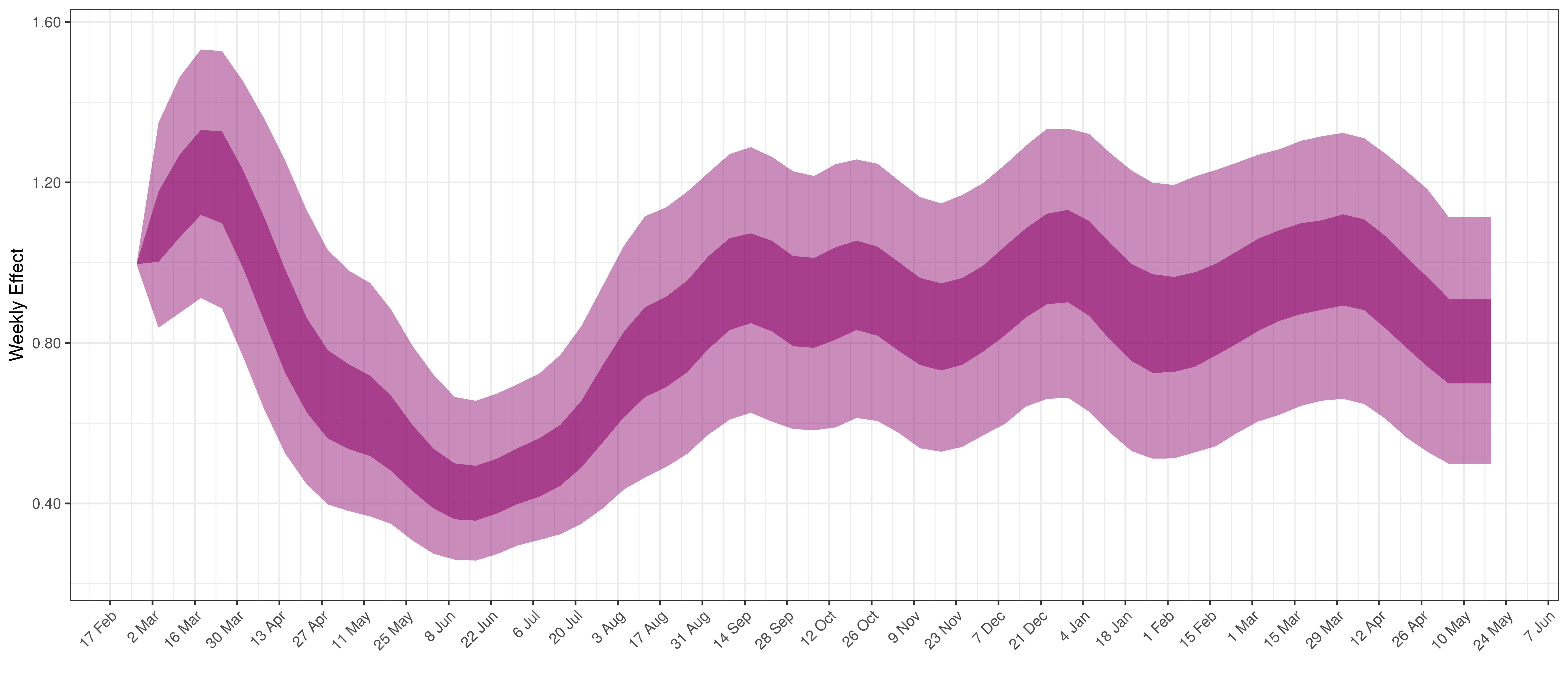
Weekly AR(2) Factor Plot for Ontario
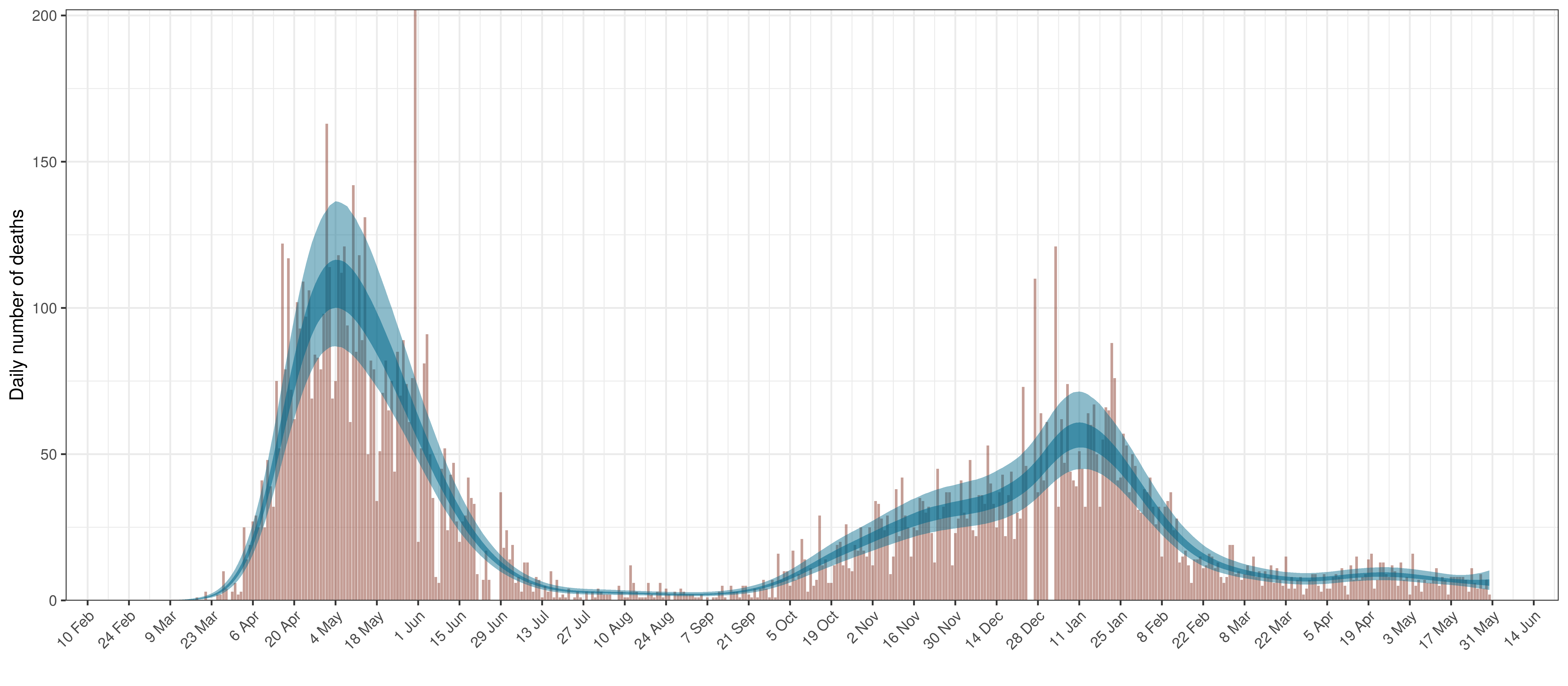
6.6 Quebec
The reported deaths (in brown) and estimated deaths (in blue) are plotted below. The calibration appears reasonable.
Projected Deaths compared to Reported COVID-19 Deaths in Quebec
Below modelled infections are plotted compared to confirmed cases. Over the last 14 days it would appear that 72.8% of all new infections were tested.
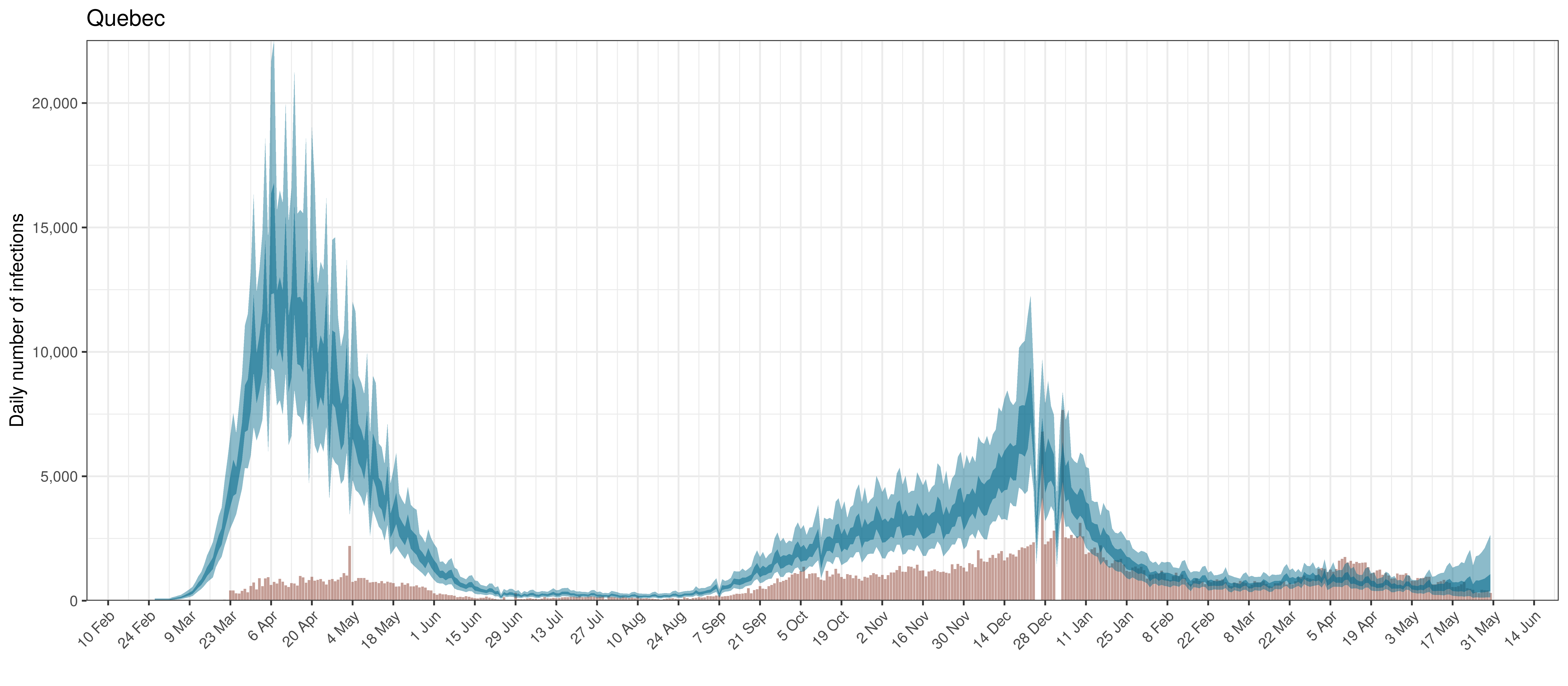
Projected Infections compared to Confirmed Cases in Quebec
Below the \(R_{t,m}\) is plotted.
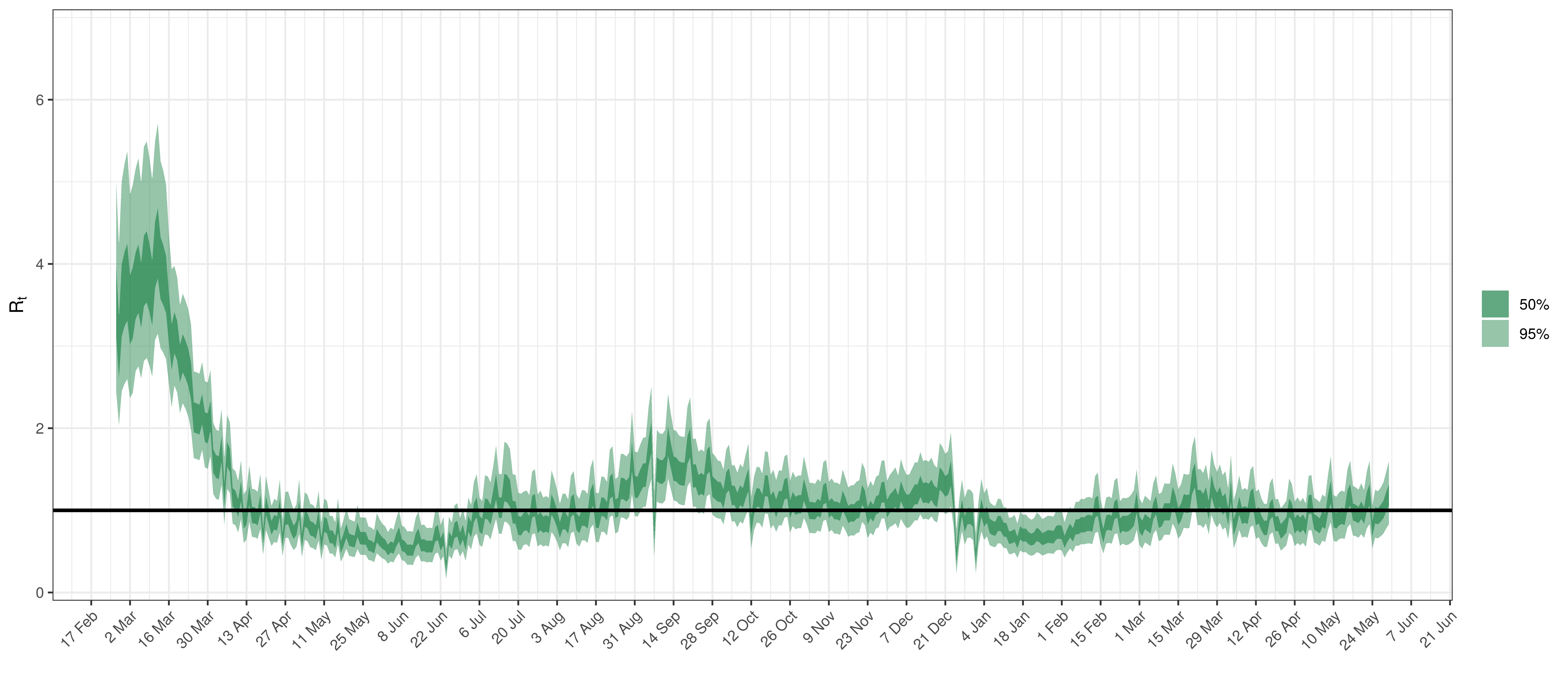
Effective Reproduction Number in Quebec
Below the \(2\cdot\phi^{-1}(-\epsilon_{w_m(t),m}))\) is plotted.
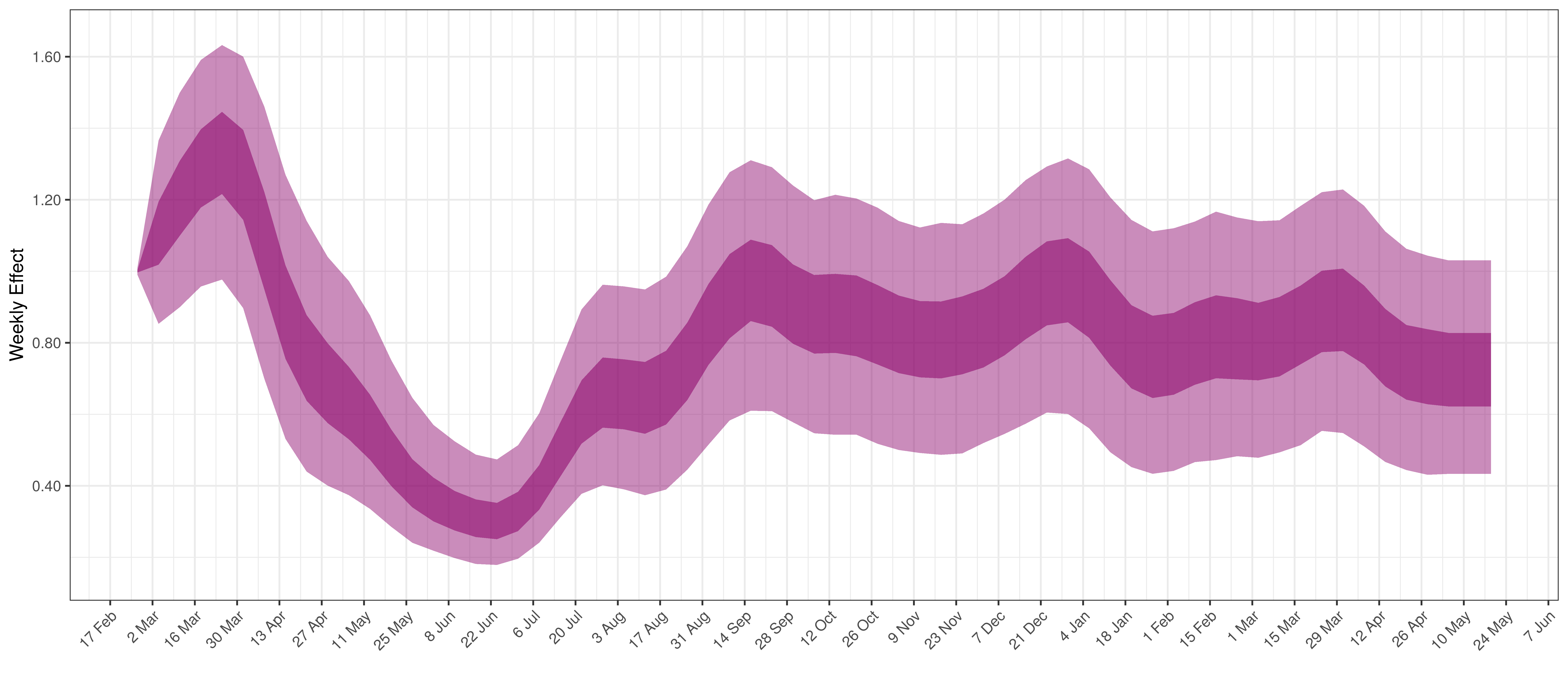
Weekly AR(2) Factor Plot for Quebec
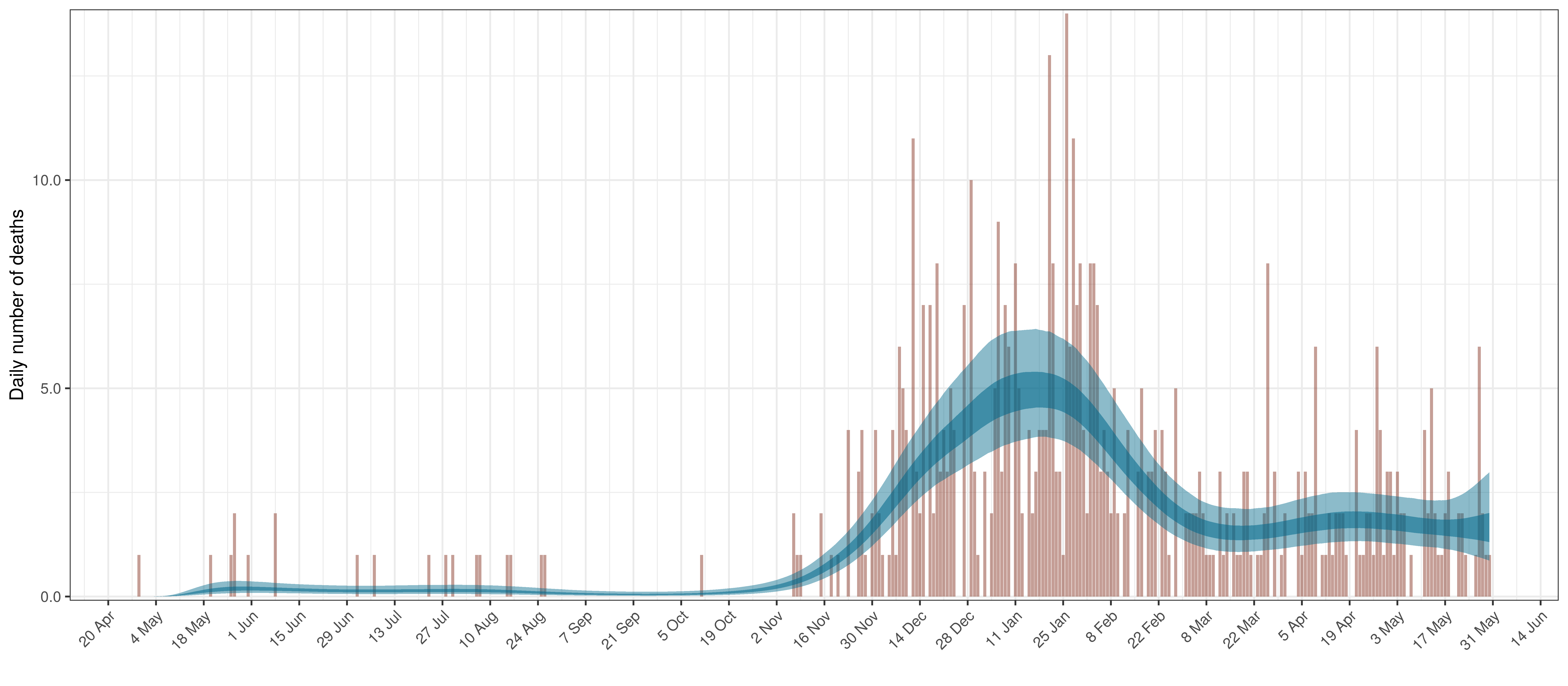
6.7 Saskatchewan
The reported deaths (in brown) and estimated deaths (in blue) are plotted below. There are somewhat limited reported deaths for this province.
Projected Deaths compared to Reported COVID-19 Deaths in Saskatchewan
Below modelled infections are plotted compared to confirmed cases. Over the last 14 days it would appear that 70.4% of all new infections were tested.
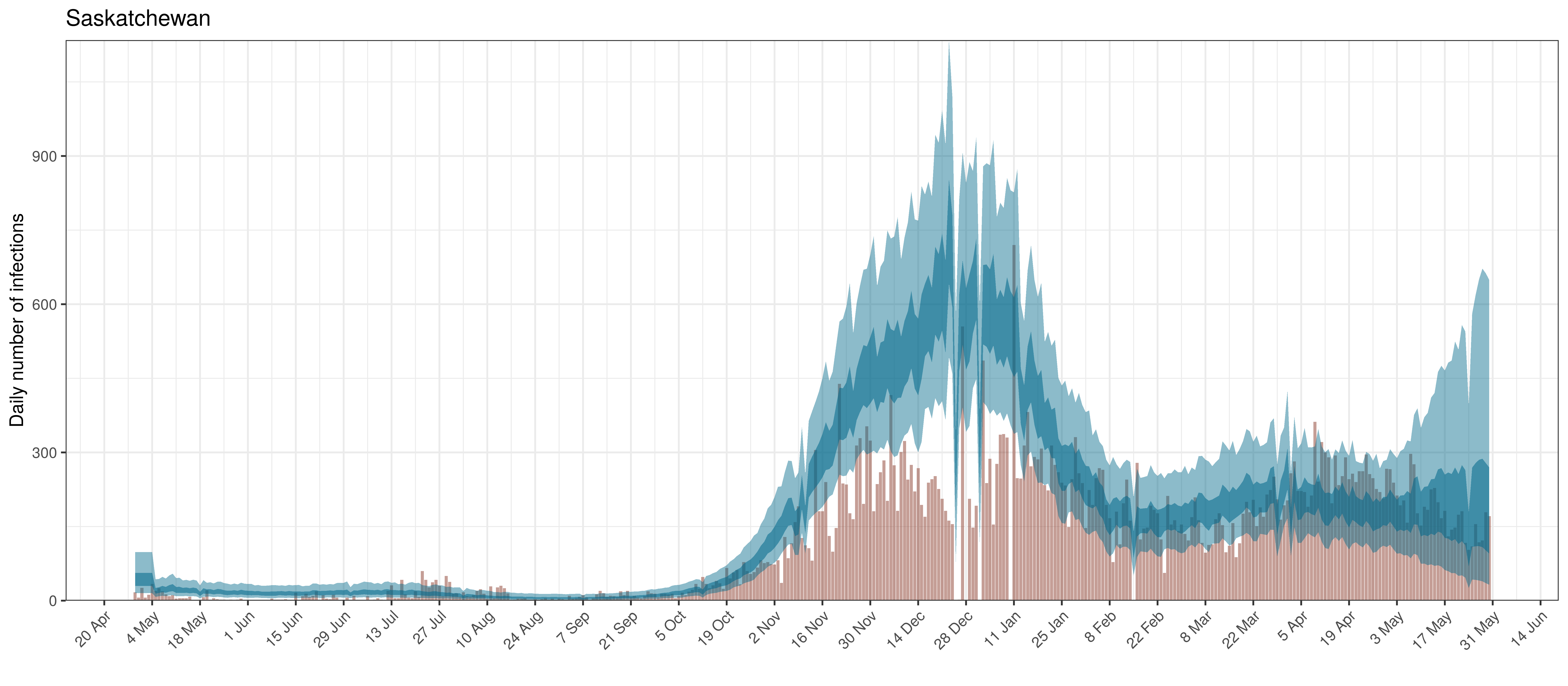
Projected Infections compared to Confirmed Cases in Saskatchewan
Below the \(R_{t,m}\) is plotted.
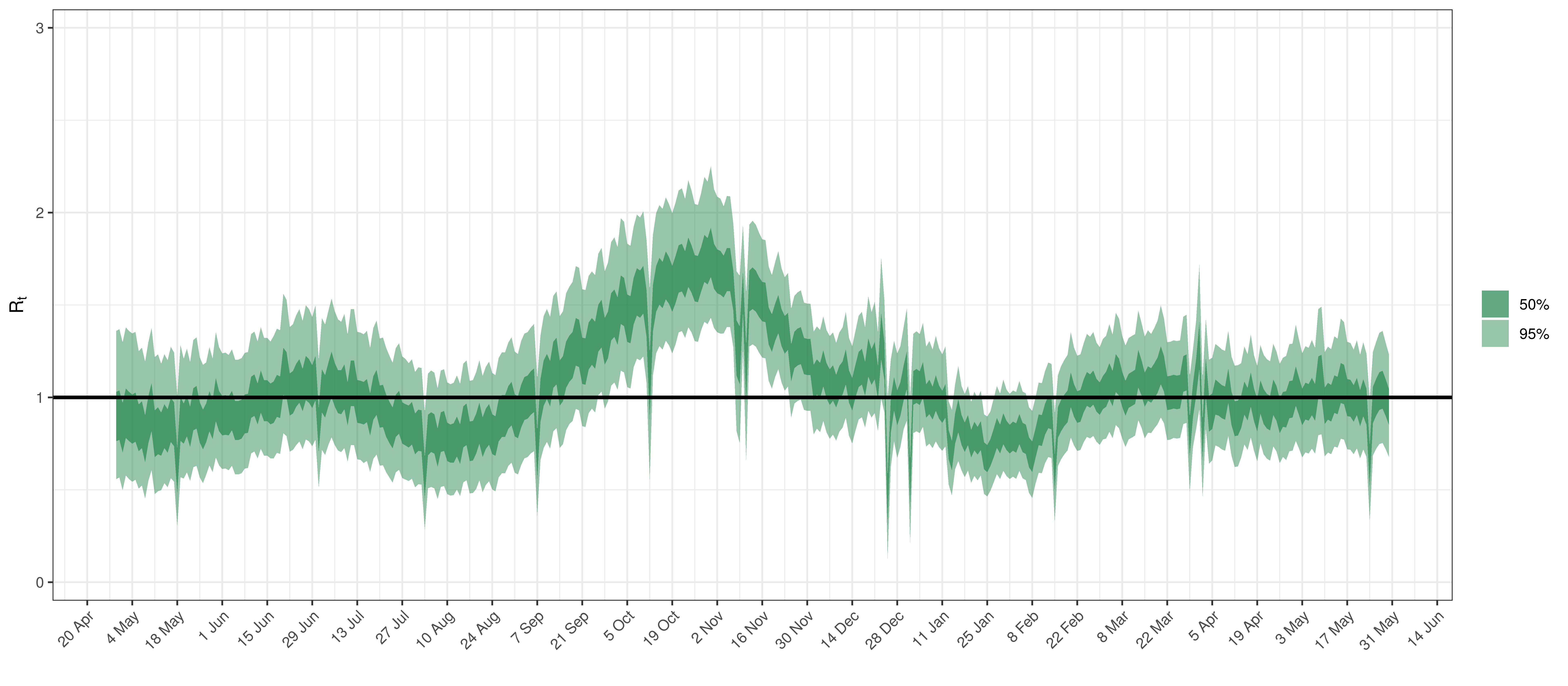
Effective Reproduction Number in Saskatchewan
Below the \(2\cdot\phi^{-1}(-\epsilon_{w_m(t),m}))\) is plotted.
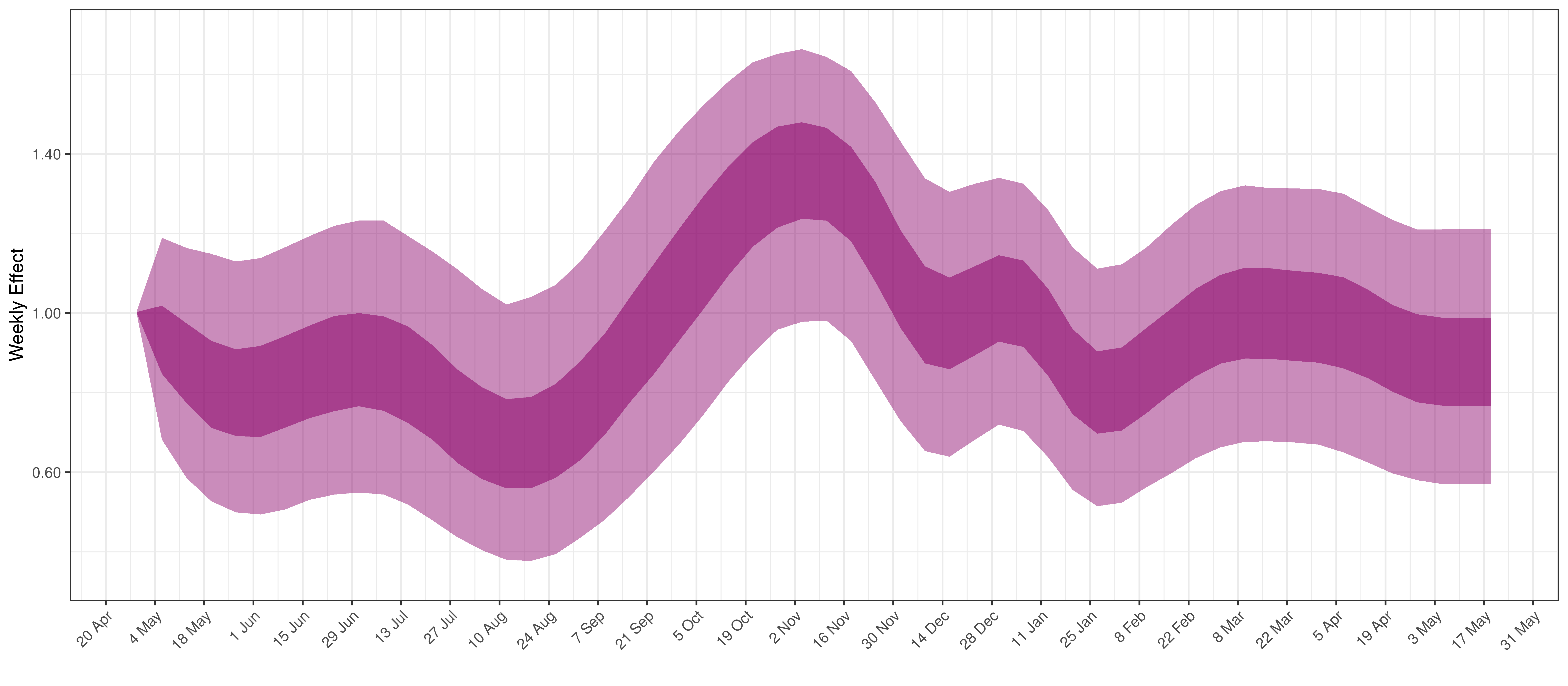
Weekly AR(2) Factor Plot for Saskatchewan
7 Parameter Estimates
To understand the net parameter estimates for \(\alpha\) and \(\alpha_{m}^s\) and their impact on \(R_{t,m}\) the percentage reduction in \(R_{t,m}\) assuming a mobility index of 0.1 (representing a 0.1 reduction in average mobility below normal). This is equivalent to plotting \(1-2\cdot\phi^{-1}(-0.1(\alpha+\alpha_{m}^s))\) for a particular province \(m\).
\(1-2\cdot\phi^{-1}(-(\beta+\beta_{m}^s))\) is also plotted. This represents the impact of mask wearing mandates on \(R_{t,m}\).
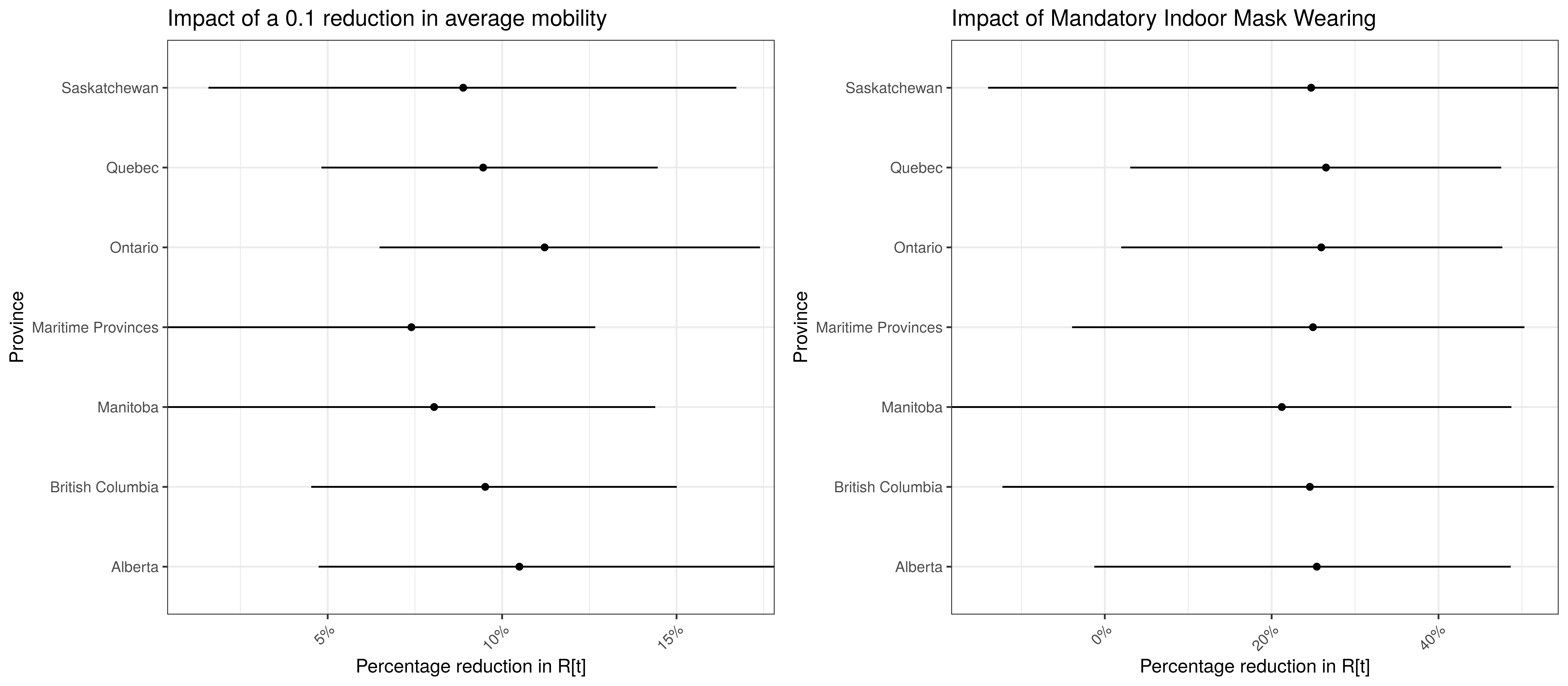
Model Parameter Estimates with 95% Confidence Intervals
8 Reproduction Number Estimates
8.1 Initial Reproduction Number
Estimates for \(R_{0,m}\) for each province are plotted below.
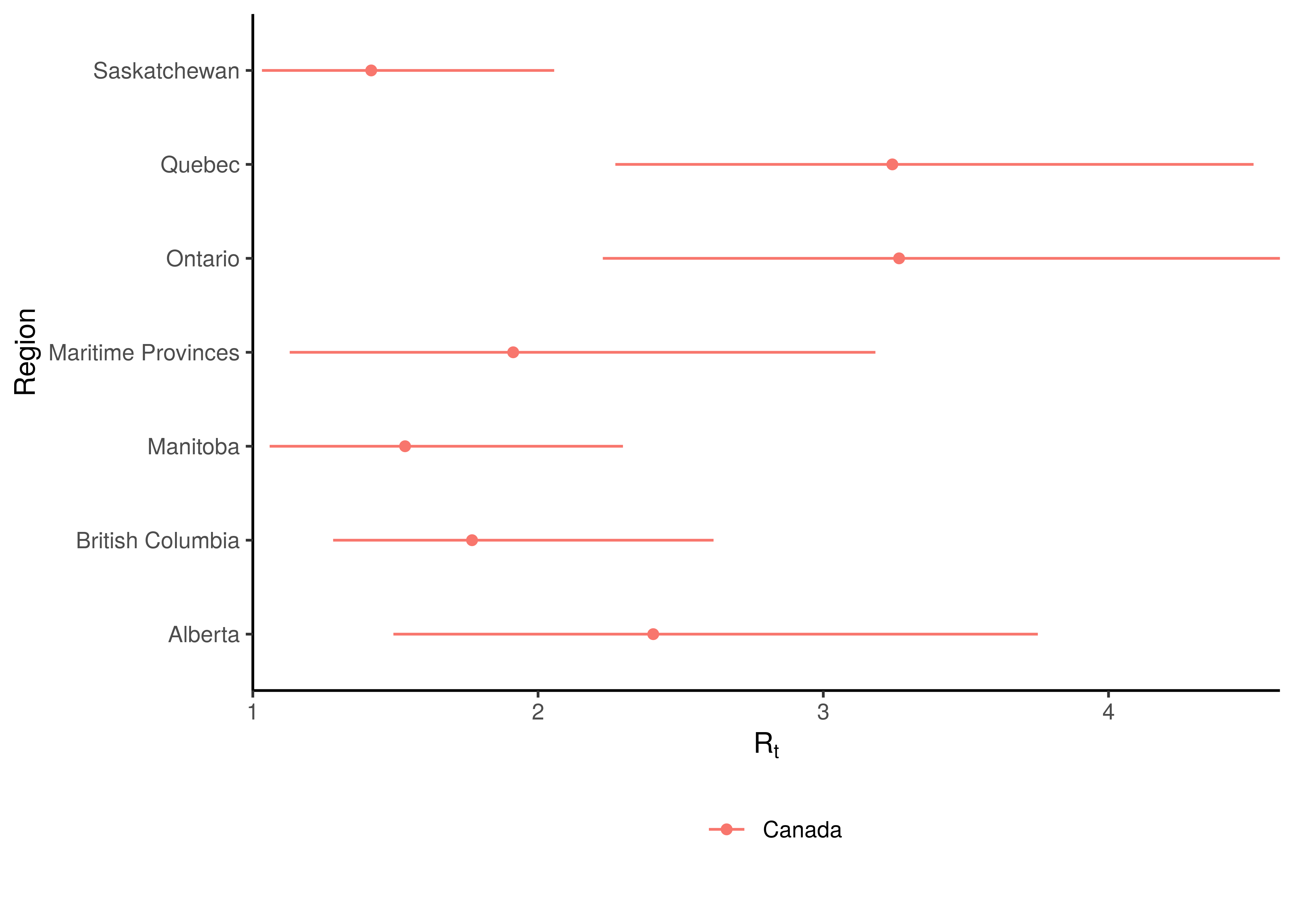
Initial Reproduction Number by Province
8.2 Current Reproduction Number as at 31 May 2021
Current estimates and 95% confidence intervals for \(R_{t,m}\) (current effective reproduction number) are plotted below for each province. A value below 1 would indicate an epidemic that is slowing while a value above 1 indicates an epidemic that is growing. It is clear that the spread of the epidemic is somewhat slowed compared to the initial \(R_{0,m}\). For some provinces the confidence interval does not include 1 which would indicate this to a stronger degree.
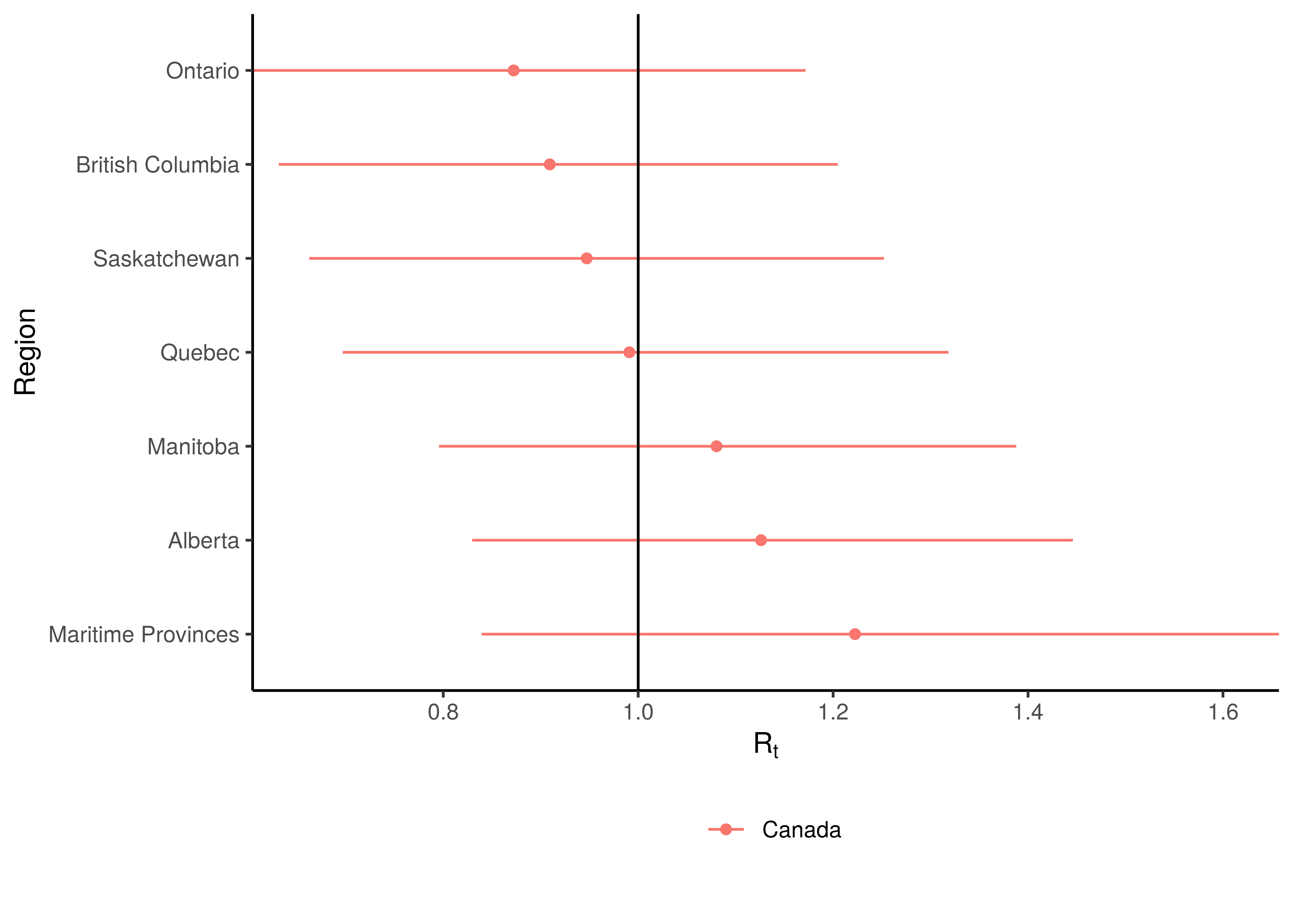
Current Reproduction Number by Province
9 Attack Rate and Cumulative Deaths as at 31 May 2021
The estimated attack rate and cumulative deaths (with 95% confidence intervals) are tabulated below (as at 31 May 2021).
The attack rate is the proportion of the population infected to date. This figure has to be estimated, because many that are infected experience no or mild symptoms, thus they may not seek medical advice and hence will never be tested.
The confidence intervals for these estimates remain wide.
| Province | Attack Rate | Cumulative Deaths |
|---|---|---|
| Alberta | 7.5% [6.0%-9.4%] | 2 237 [ 2 036 - 2 462] |
| British Columbia | 3.4% [2.8%-4.3%] | 1 700 [ 1 546 - 1 867] |
| Manitoba | 9.9% [7.8%-12.7%] | 1 052 [ 936 - 1 181] |
| Maritime Provinces | 0.6% [0.5%-1.0%] | 132 [ 108 - 158] |
| Ontario | 6.5% [5.3%-8.2%] | 8 756 [ 8 136 - 9 415] |
| Quebec | 12.9% [10.4%-16.2%] | 11 233 [10 341 - 12 228] |
| Saskatchewan | 5.6% [4.4%-7.1%] | 536 [ 475 - 607] |
| Canada | 7.4% [6.6%-8.4%] | 25 645 [24 494 - 26 890] |
10 Projections
One of the reasons we build models is so that we can make sense of the future or indeed the past. We can project forward models to assess the impact of varying assumptions on future outcomes. This gives us a sense of how changes in actions may impact the future. I.e. it allows us to answer “what if” questions. Note however that in projecting the future we are extrapolating, and due care needs to be taken. There are numerous limitations to this model and these projections dicussed below but the author is also of the opinion that the projections add value in that they indicate a significant range across the scenarios projected and in such a manner inform discussion.
All models are wrong but some are useful - George Box [9]
An incorrect model can be useful because it enables a better understanding of the model and the phenomena being modelled.
Note detailed projection output can be found here.
Projections are done using constant, increasing and decreasing mobility but other interventions are left constant. It should also be noted that the \(\epsilon_{w_m(t),m}\) are projected forward at constant levels and are not adjusted for projection purposes.
The \(\epsilon_{w_m(t),m}\) is held at “current” levels when projecting forwards. It should be noted that these levels are set 28 days prior as recent deaths only affect infections that occured prior to that. Based on the observed calibration for Western Cape there is a possibility that this may be resulting in too low recent infections.
10.1 No change in Mobility
In this projection mobility is held constant at current levels. Mask wearing interventions are left intact.
The result of this scenario as at 30 June 2021 and 30 September 2021 are tabulated below.
| Province | Attack Rate | Deaths | Peak Daily Deaths | Peak Date |
|---|---|---|---|---|
| Alberta | 9.2% [6.5%-15.4%] | 2 534 [ 2 209- 3 062] | 49 | 2021-09-08 |
| British Columbia | 3.6% [2.8%-4.8%] | 1 805 [ 1 624- 2 040] | 15 | 2020-12-16 |
| Manitoba | 12.3% [8.5%-20.2%] | 1 224 [ 1 043- 1 518] | 16 | 2021-08-25 |
| Maritime Provinces | 1.6% [0.5%-5.7%] | 219 [ 136- 424] | 72 | 2021-09-19 |
| Ontario | 6.8% [5.4%-9.0%] | 9 213 [ 8 463-10 167] | 57 | 2021-01-15 |
| Quebec | 13.3% [10.6%-17.0%] | 11 455 [10 521-12 518] | 109 | 2020-05-05 |
| Saskatchewan | 6.2% [4.5%-9.2%] | 593 [ 508- 708] | 5 | 2021-01-17 |
| Canada | 8.0% [6.9%-9.3%] | 27 042 [25 716-28 634] | 217 | 2021-09-20 |
| Province | Attack Rate | Deaths | Peak Daily Deaths | Peak Date |
|---|---|---|---|---|
| Alberta | 21.2% [7.0%-56.6%] | 5 963 [ 2 360- 17 213] | 49 | 2021-09-08 |
| British Columbia | 4.9% [2.9%-16.4%] | 2 331 [ 1 657- 5 999] | 15 | 2020-12-16 |
| Manitoba | 22.7% [8.9%-54.5%] | 2 428 [ 1 118- 6 074] | 16 | 2021-08-25 |
| Maritime Provinces | 20.9% [0.6%-67.3%] | 4 233 [ 162- 17 730] | 72 | 2021-09-19 |
| Ontario | 8.4% [5.5%-22.1%] | 11 155 [ 8 602- 24 050] | 57 | 2021-01-15 |
| Quebec | 17.1% [10.9%-45.4%] | 14 049 [10 717- 31 154] | 109 | 2020-05-05 |
| Saskatchewan | 9.2% [4.6%-30.0%] | 870 [ 523- 2 483] | 5 | 2021-01-17 |
| Canada | 12.8% [8.1%-21.8%] | 41 029 [28 795- 68 553] | 217 | 2021-09-20 |
10.2 Increase in mobility
This scenario assumes future mobility increases by a fixed value of 0.1. Other interventions are left intact. The attack rate and deaths after increasing mobility are tabulated below (as at 30 June 2021 and 30 September 2021).
| Province | Attack Rate | Deaths | Peak Daily Deaths | Peak Date |
|---|---|---|---|---|
| Alberta | 10.4% [6.6%-21.2%] | 2 579 [ 2 222- 3 228] | 119 | 2021-08-27 |
| British Columbia | 3.7% [2.9%-5.3%] | 1 814 [ 1 626- 2 063] | 38 | 2021-10-14 |
| Manitoba | 13.0% [8.6%-22.8%] | 1 236 [ 1 046- 1 556] | 27 | 2021-08-26 |
| Maritime Provinces | 2.0% [0.5%-8.1%] | 229 [ 138- 471] | 114 | 2021-09-08 |
| Ontario | 7.2% [5.5%-10.4%] | 9 269 [ 8 483-10 363] | 162 | 2021-09-21 |
| Quebec | 13.6% [10.7%-17.8%] | 11 483 [10 537-12 589] | 154 | 2021-09-22 |
| Saskatchewan | 6.5% [4.6%-10.3%] | 597 [ 509- 722] | 10 | 2021-09-19 |
| Canada | 8.4% [7.1%-10.5%] | 27 207 [25 820-28 954] | 597 | 2021-09-13 |
Based on the above an increase mobility could mean roughly 0 more deaths by end of June 2021.
| Province | Attack Rate | Deaths | Peak Daily Deaths | Peak Date |
|---|---|---|---|---|
| Alberta | 37.3% [7.7%-74.2%] | 10 534 [ 2 495- 24 492] | 119 | 2021-08-27 |
| British Columbia | 8.5% [3.0%-43.5%] | 3 572 [ 1 677- 16 172] | 38 | 2021-10-14 |
| Manitoba | 30.6% [9.6%-62.9%] | 3 213 [ 1 161- 7 326] | 27 | 2021-08-26 |
| Maritime Provinces | 32.3% [0.7%-76.3%] | 6 909 [ 183- 20 941] | 114 | 2021-09-08 |
| Ontario | 15.9% [5.7%-62.2%] | 18 792 [ 8 729- 76 668] | 162 | 2021-09-21 |
| Quebec | 26.1% [11.3%-69.4%] | 19 875 [10 871- 57 055] | 154 | 2021-09-22 |
| Saskatchewan | 13.9% [4.8%-51.3%] | 1 237 [ 532- 4 622] | 10 | 2021-09-19 |
| Canada | 21.2% [9.9%-42.9%] | 64 131 [32 860-133 176] | 597 | 2021-09-13 |
Based on the above an increase mobility could mean roughly 23 000 more deaths by the end of September 2021.
10.3 Decreased mobility
This scenario assumes future mobility decreases by a fixed value of 0.1. The attack rate and deaths after decreased mobility are tabulated below (as at 30 June 2021 and 30 September 2021).
| Province | Attack Rate | Deaths | Peak Daily Deaths | Peak Date |
|---|---|---|---|---|
| Alberta | 8.6% [6.3%-13.0%] | 2 504 [ 2 199- 2 970] | 23 | 2021-01-05 |
| British Columbia | 3.6% [2.8%-4.6%] | 1 799 [ 1 621- 2 023] | 15 | 2020-12-16 |
| Manitoba | 11.8% [8.3%-18.6%] | 1 214 [ 1 040- 1 489] | 13 | 2020-12-05 |
| Maritime Provinces | 1.3% [0.5%-4.4%] | 211 [ 136- 394] | 44 | 2021-09-24 |
| Ontario | 6.7% [5.4%-8.6%] | 9 178 [ 8 447-10 067] | 57 | 2021-01-15 |
| Quebec | 13.2% [10.5%-16.6%] | 11 436 [10 510-12 483] | 109 | 2020-05-05 |
| Saskatchewan | 6.0% [4.5%-8.5%] | 590 [ 508- 699] | 5 | 2021-01-17 |
| Canada | 7.8% [6.8%-9.0%] | 26 932 [25 646-28 444] | 169 | 2020-05-02 |
Based on the above a decrease in mobility could mean roughly 0 fewer deaths by end of June 2021.
| Province | Attack Rate | Deaths | Peak Daily Deaths | Peak Date |
|---|---|---|---|---|
| Alberta | 13.1% [6.5%-41.5%] | 3 920 [ 2 280- 11 597] | 23 | 2021-01-05 |
| British Columbia | 4.0% [2.9%-8.2%] | 2 017 [ 1 643- 3 501] | 15 | 2020-12-16 |
| Manitoba | 18.2% [8.6%-50.0%] | 1 998 [ 1 087- 5 425] | 13 | 2020-12-05 |
| Maritime Provinces | 12.9% [0.5%-60.7%] | 2 598 [ 151- 14 764] | 44 | 2021-09-24 |
| Ontario | 7.1% [5.4%-10.5%] | 9 742 [ 8 535- 13 265] | 57 | 2021-01-15 |
| Quebec | 14.4% [10.7%-26.4%] | 12 381 [10 622- 19 232] | 109 | 2020-05-05 |
| Saskatchewan | 7.4% [4.6%-19.8%] | 733 [ 518- 1 658] | 5 | 2021-01-17 |
| Canada | 9.8% [7.3%-15.1%] | 33 389 [27 037- 49 541] | 169 | 2020-05-02 |
Based on the above a decrease in mobility could mean roughly 8 000 fewer deaths by the end of September 2021.
10.4 Worst Case Scenario
This scenario assumes future mobility increases by a fixed value of 0.1, mask wearing is eliminated as well as that the AR(2) term reverts to 0. The attack rate and deaths are tabulated below (as at 30 June 2021 and 30 September 2021). This would be a relatively extreme worst case scenario as this essentially assumes not mitigation measures in place and would probably be close to the absolute worst case.
| Province | Attack Rate | Deaths | Peak Daily Deaths | Peak Date |
|---|---|---|---|---|
| Alberta | 15.7% [7.1%-45.7%] | 2 716 [ 2 250- 3 754] | 295 | 2021-08-09 |
| British Columbia | 3.7% [2.9%-5.3%] | 1 814 [ 1 626- 2 063] | 38 | 2021-10-14 |
| Manitoba | 14.6% [8.8%-29.0%] | 1 257 [ 1 054- 1 617] | 50 | 2021-08-19 |
| Maritime Provinces | 5.5% [0.6%-32.8%] | 285 [ 143- 771] | 270 | 2021-08-16 |
| Ontario | 10.0% [5.8%-27.4%] | 9 552 [ 8 554-11 544] | 1 019 | 2021-08-19 |
| Quebec | 16.6% [11.2%-34.8%] | 11 654 [10 600-13 102] | 734 | 2021-08-16 |
| Saskatchewan | 6.5% [4.6%-10.3%] | 597 [ 509- 722] | 10 | 2021-09-19 |
| Canada | 11.0% [7.7%-20.3%] | 27 874 [26 106-30 701] | 2 376 | 2021-08-16 |
Based on the above the worst case scenario could result in roughly 1 000 more deaths by the end of June 2021.
| Province | Attack Rate | Deaths | Peak Daily Deaths | Peak Date |
|---|---|---|---|---|
| Alberta | 64.7% [12.2%-90.1%] | 19 848 [ 3 385- 31 345] | 295 | 2021-08-09 |
| British Columbia | 8.5% [3.0%-43.5%] | 3 572 [ 1 677- 16 172] | 38 | 2021-10-14 |
| Manitoba | 43.6% [10.7%-74.8%] | 4 648 [ 1 243- 9 097] | 50 | 2021-08-19 |
| Maritime Provinces | 64.1% [2.4%-93.4%] | 15 972 [ 460- 27 305] | 270 | 2021-08-16 |
| Ontario | 56.0% [6.8%-91.1%] | 70 696 [ 9 424-135 550] | 1 019 | 2021-08-19 |
| Quebec | 65.9% [13.6%-93.0%] | 53 964 [11 814- 89 636] | 734 | 2021-08-16 |
| Saskatchewan | 13.9% [4.8%-51.3%] | 1 237 [ 532- 4 622] | 10 | 2021-09-19 |
| Canada | 51.6% [20.6%-73.1%] | 169 937 [61 264-267 863] | 2 376 | 2021-08-16 |
Based on the above the worst case scenario could result in roughly 129 000 more deaths by the end of September 2021.
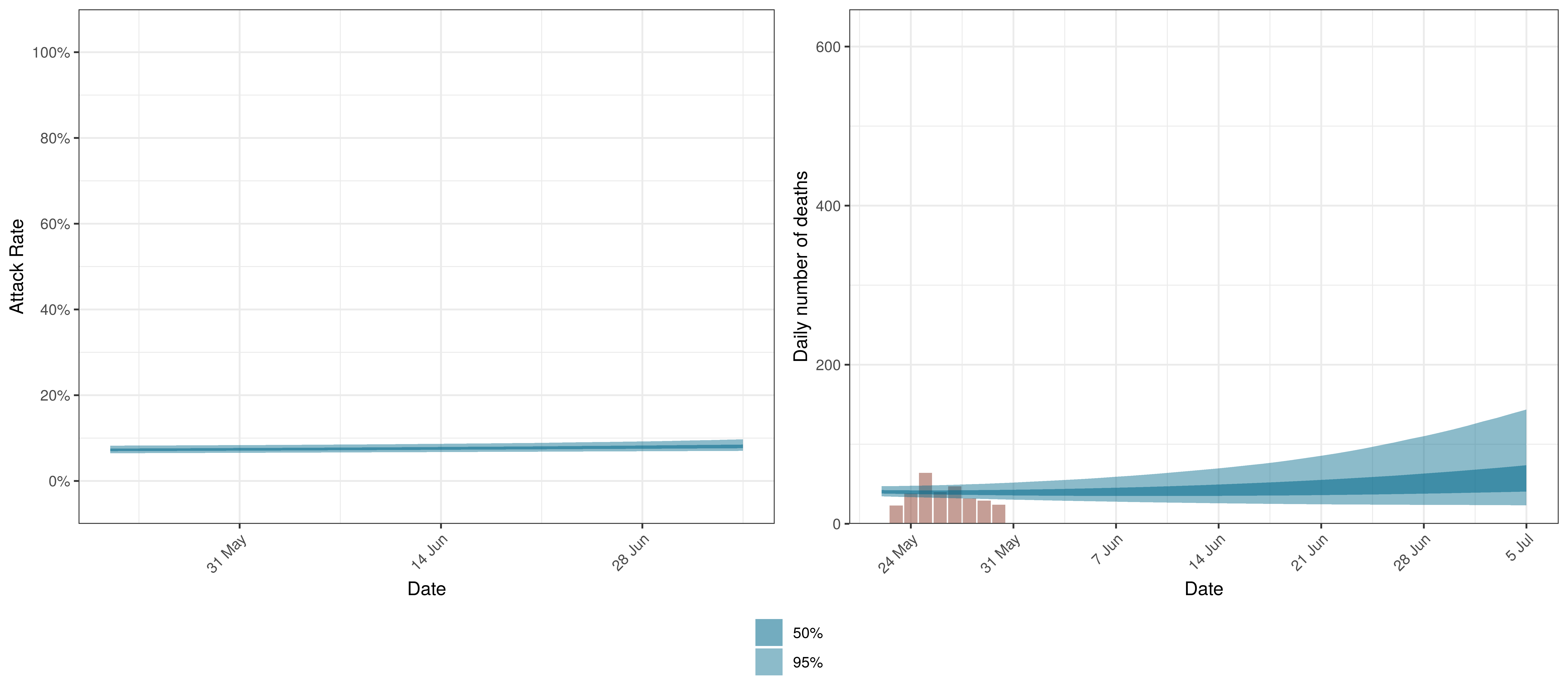
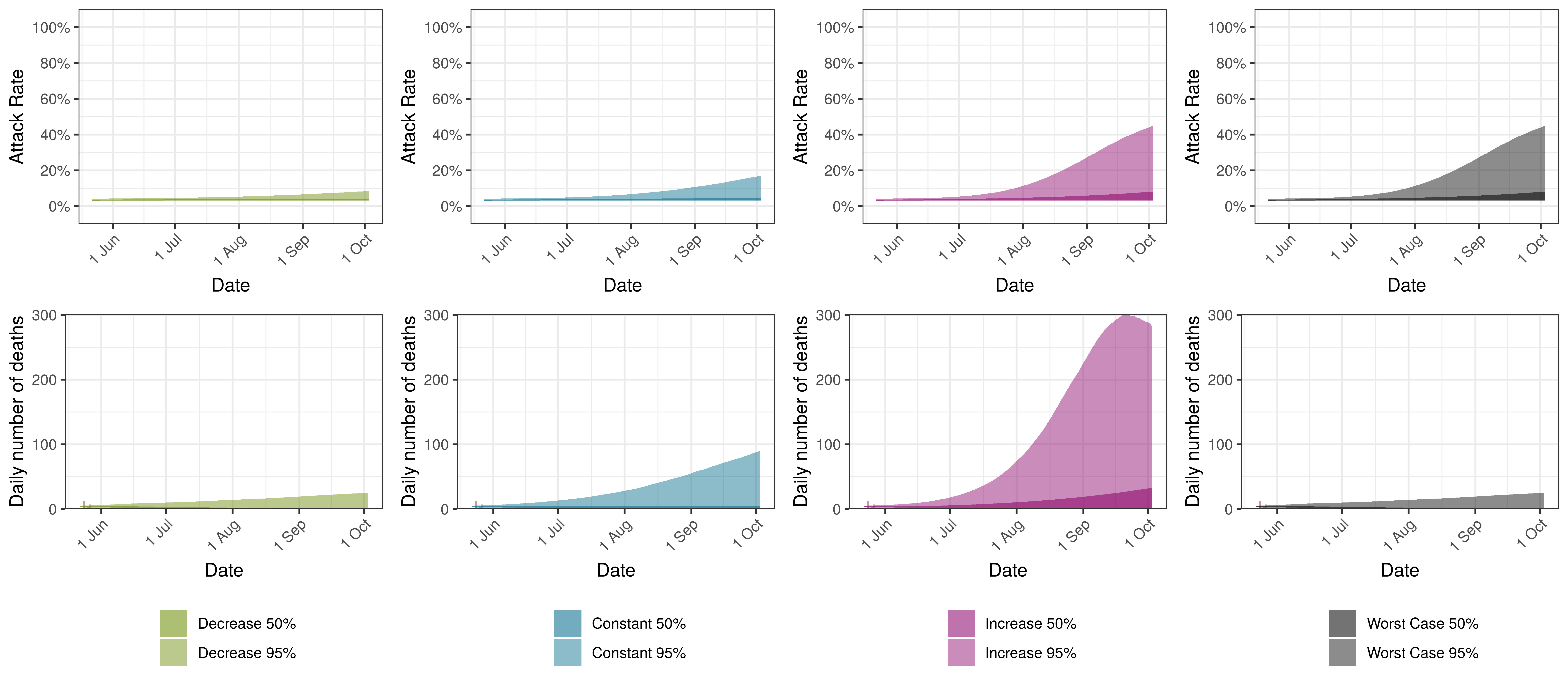
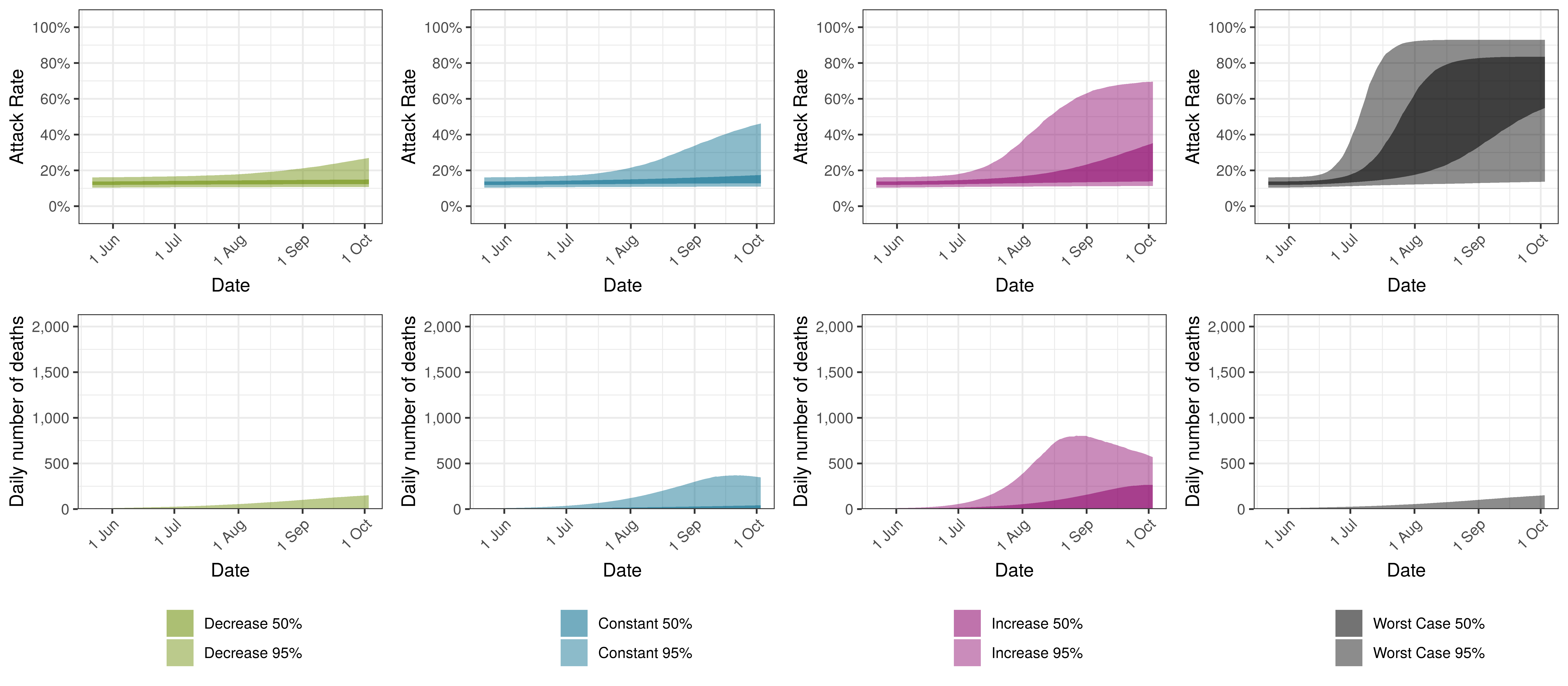
10.5 Canada
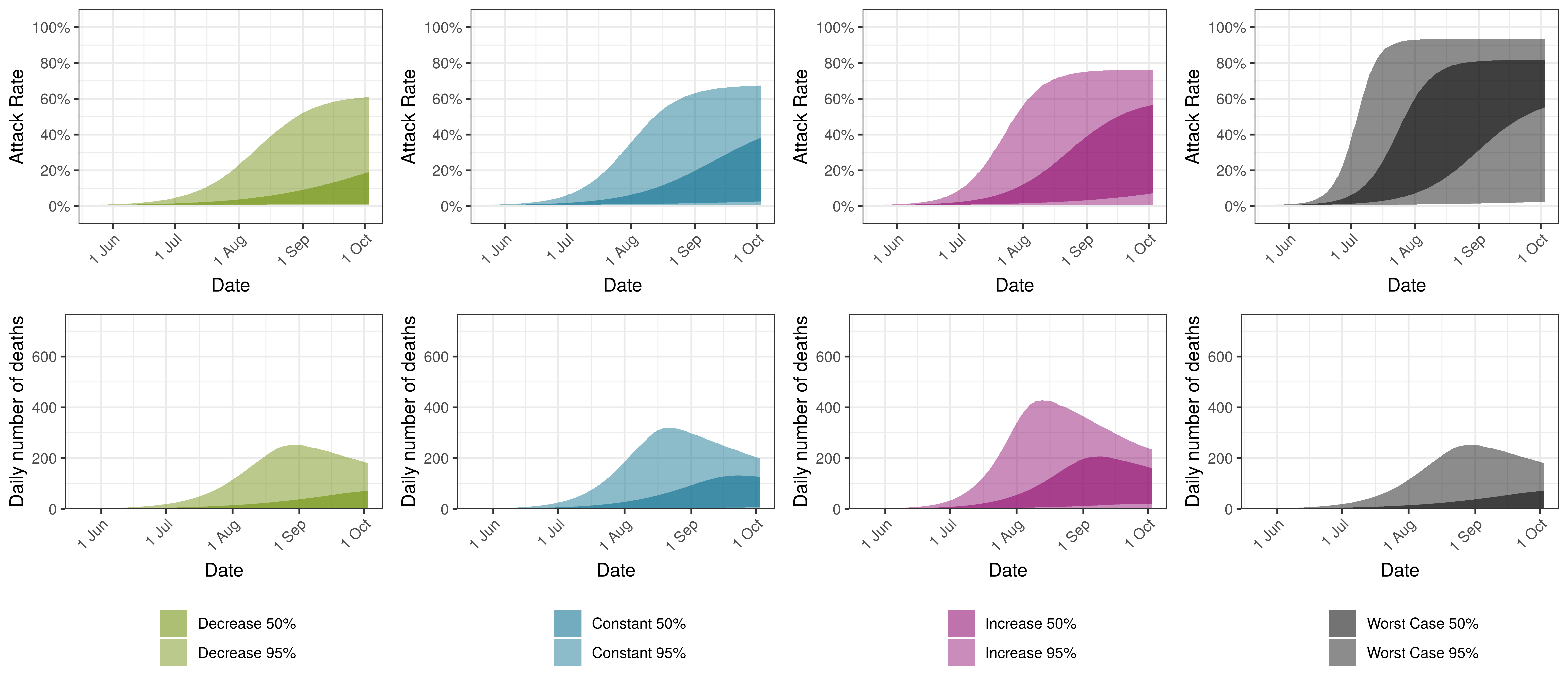
We plot below the results for Canada as a whole. This is the sum of the provincial projections.
Projected Attack Rate and Daily Deaths in Canada
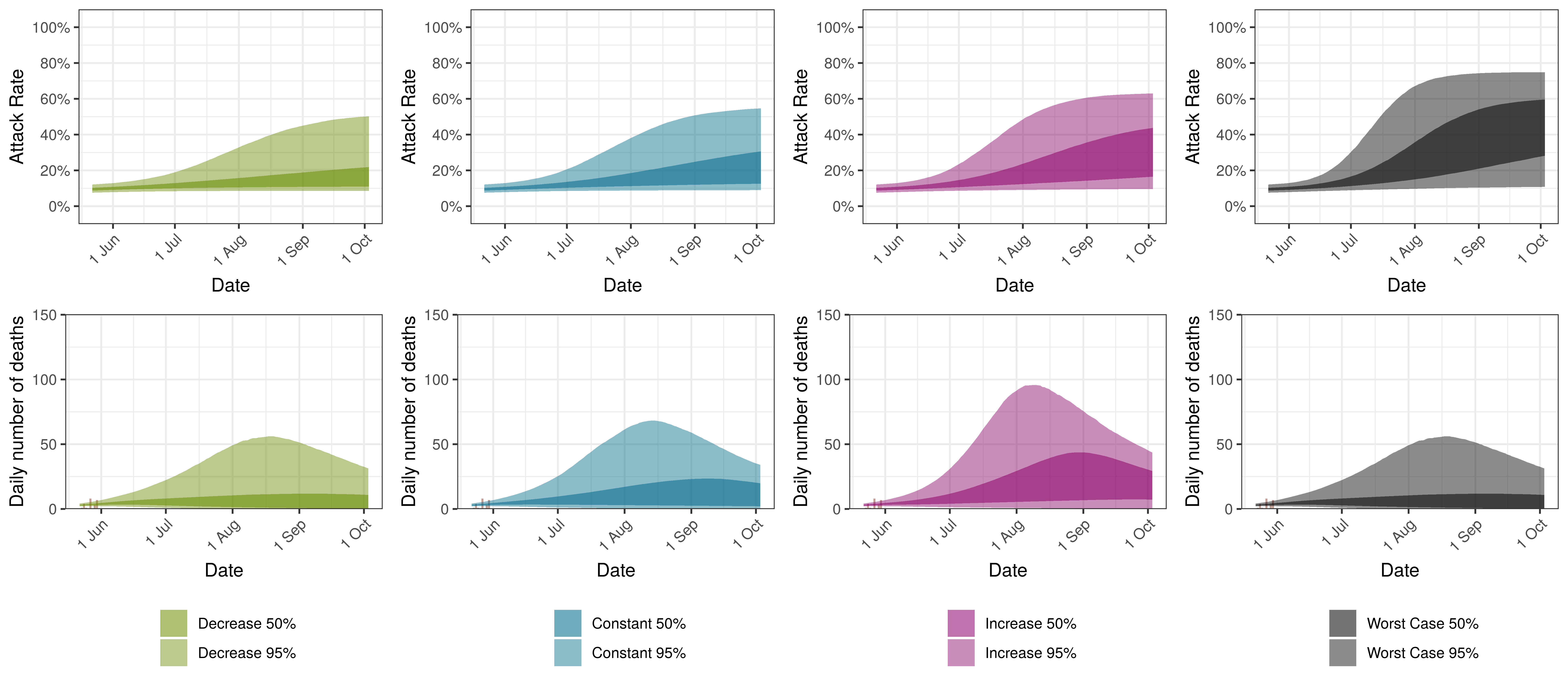
The attack rate and deaths over a longer period for both the constant mobility and increased mobility scenarios are plotted below:
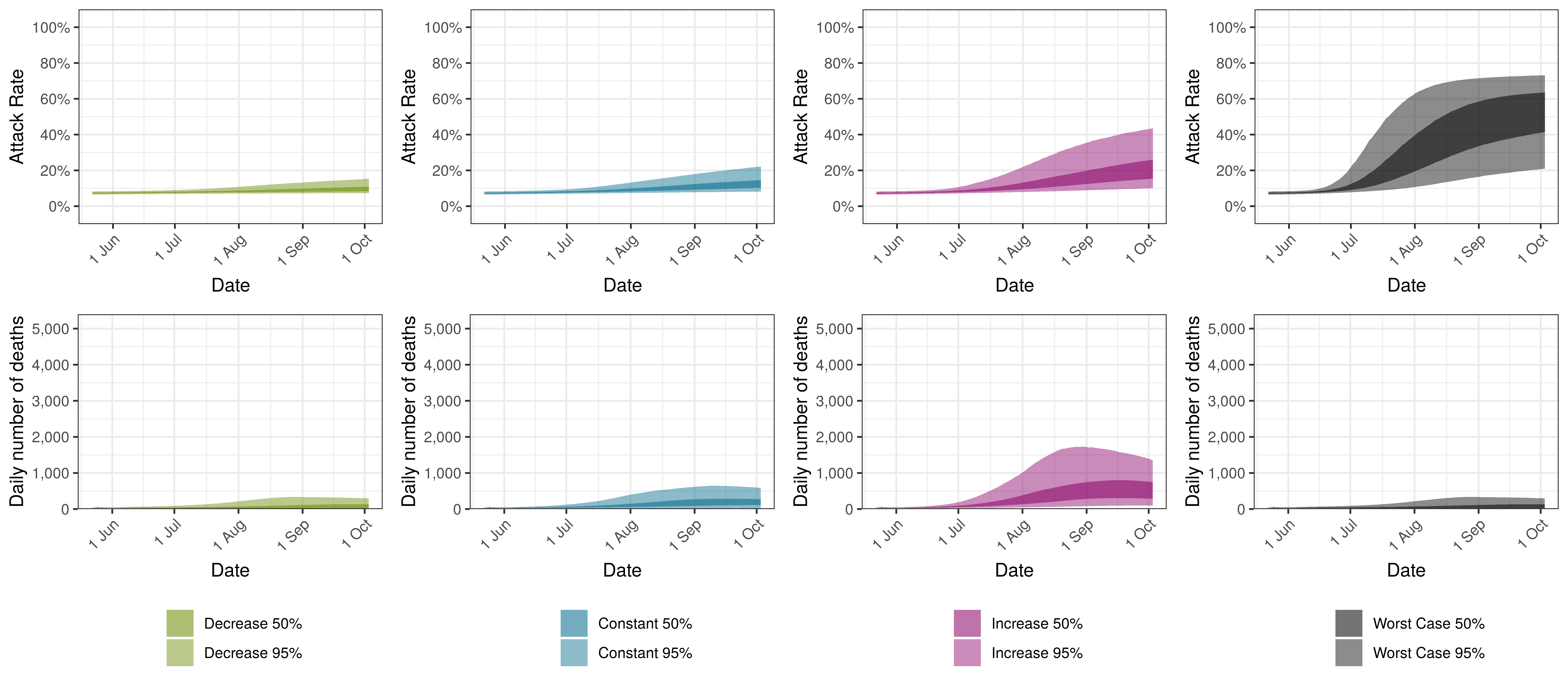
Projected Attack Rate and Daily Deaths in Canada by Scenario
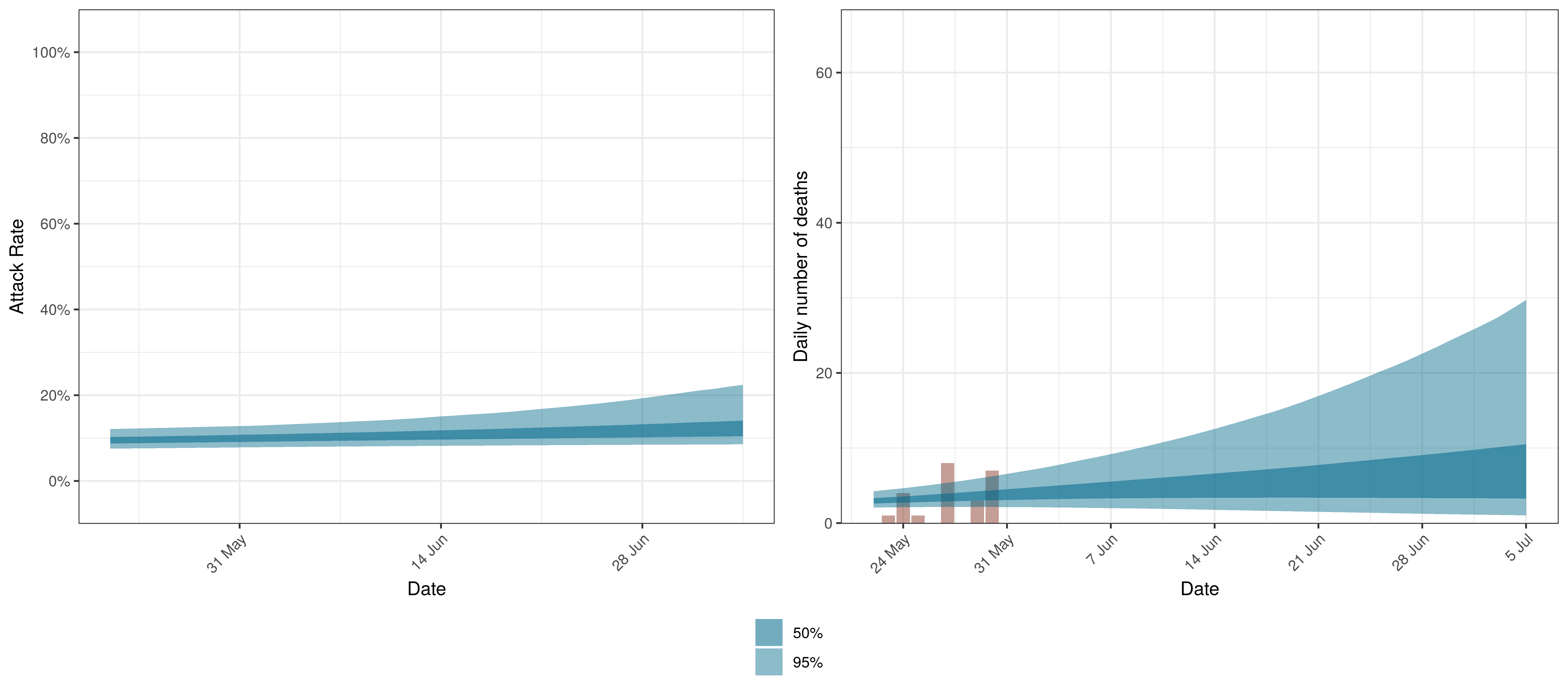
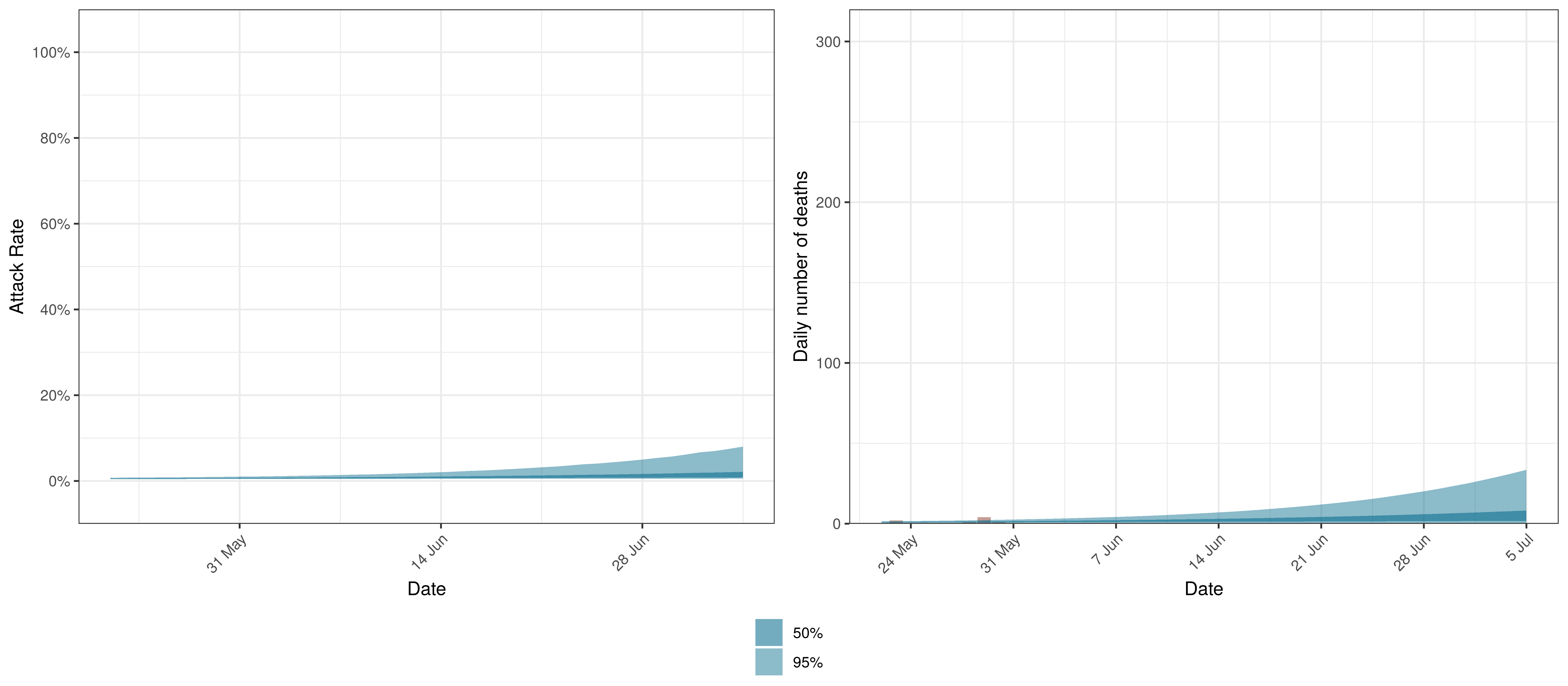
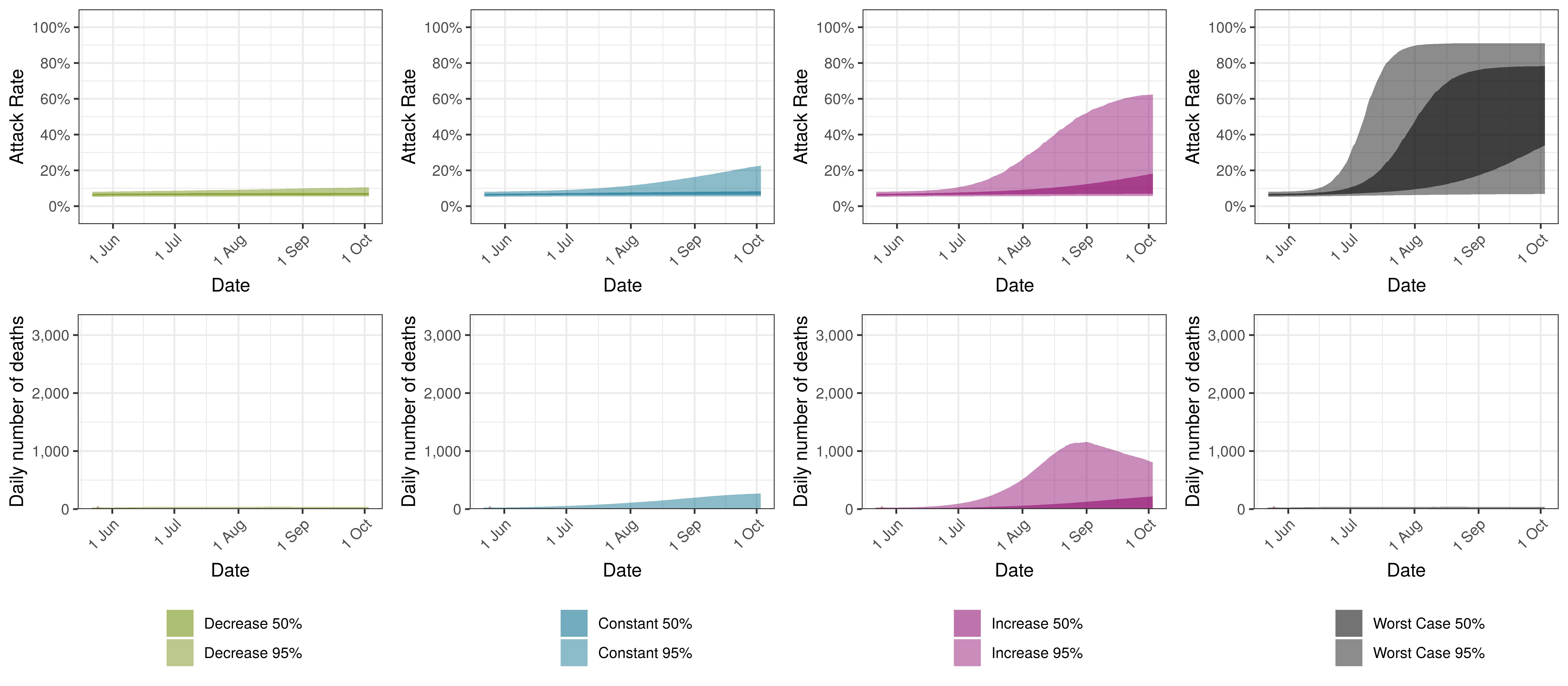
10.6 Alberta
Below we plot the projections for Alberta.
Projected Attack Rate and Daily Deaths in Alberta
The attack rate and deaths over a longer period for both the constant mobility and increased mobility scenarios are plotted below:
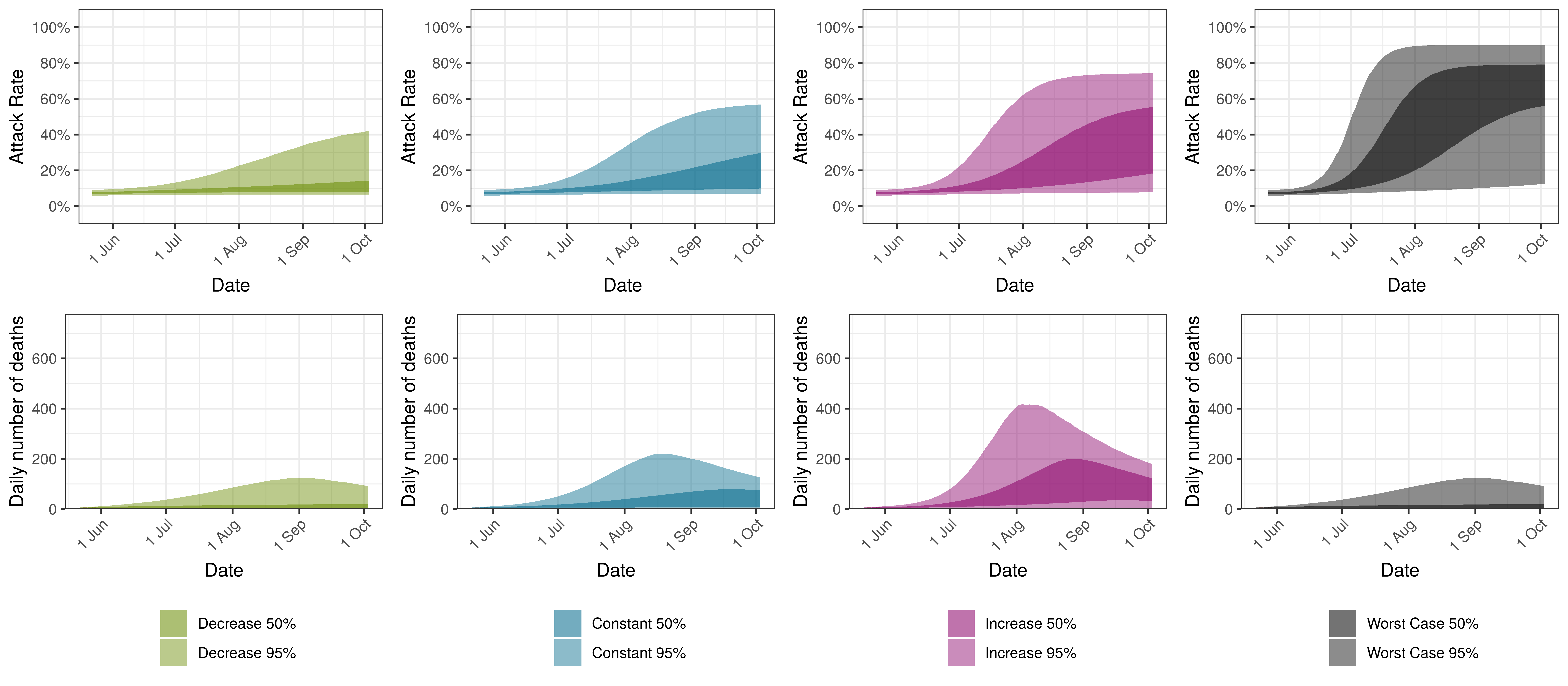
Projected Attack Rate and Daily Deaths in Alberta by Scenario
10.7 British Columbia
Below we plot the projections for the British Columbia.
Projected Attack Rate and Daily Deaths in British Columbia
The attack rate and deaths over a longer period for both the constant mobility and increased mobility scenarios are plotted below:
Projected Attack Rate and Daily Deaths in British Columbia by Scenario
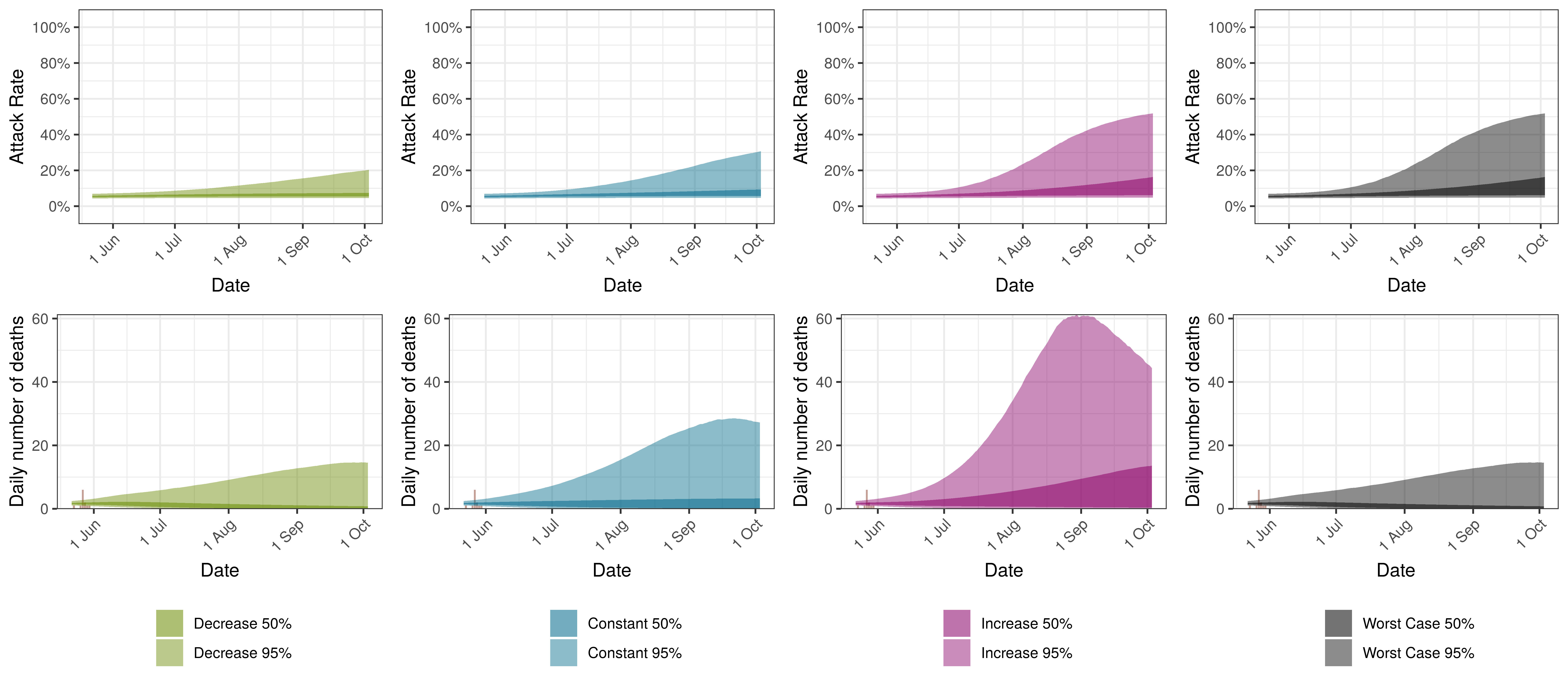
10.8 Manitoba
Below we plot the projections for Manitoba
Projected Attack Rate and Daily Deaths in Manitoba
The attack rate and deaths over a longer period for both the constant mobility and increased mobility scenarios are plotted below:
Projected Attack Rate and Daily Deaths in Manitoba by Scenario
10.9 Maritime Provinces
Below we plot the projections for Maritime Provinces
Projected Attack Rate and Daily Deaths in Maritime Provinces
The attack rate and deaths over a longer period for both the constant mobility and increased mobility scenarios are plotted below:
Projected Attack Rate and Daily Deaths in Maritime Provinces by Scenario
10.10 Ontario
Below we plot the projections for Ontario.
Projected Attack Rate and Daily Deaths in Ontario
The attack rate and deaths over a longer period for both the constant mobility and increased mobility scenarios are plotted below:
Projected Attack Rate and Daily Deaths in Ontario by Scenario
10.11 Quebec
Below we plot the projections for Quebec.
Projected Attack Rate and Daily Deaths in Quebec
The attack rate and deaths over a longer period for both the constant mobility and increased mobility scenarios are plotted below:
Projected Attack Rate and Daily Deaths in Quebec by Scenario
10.12 Saskatchewan
Below we plot the projections for Saskatchewan.
Projected Attack Rate and Daily Deaths in Saskatchewan
The attack rate and deaths over a longer period for both the constant mobility and increased mobility scenarios are plotted below:
Projected Attack Rate and Daily Deaths in Saskatchewan by Scenario
11 Discussion
There remains significant uncertainty with all matters relating this epidemic. This includes uncertainty in data, assumptions and many epidemiological and medical matters relating to this disease. It is therefore likely that the model will not be accurate. It is also reflected in the wide confidence intervals of many of the results of the model.
Some researchers have gone as far as to say that it is not possible to accurately estimate the mean number of fatalities of pandemics based on data ([10] & [11]). This would indicate the goal of the paper may be futile.
This paper has however attempted to allow for uncertainty using the Bayesian approach here which results in at least some distribution of possible results, some of which are definitely catastrophic and some of which are less severe.
11.1 Limitations
This analysis has various limitations. We highlight a few below but there are many. Perhaps the most important being the lack of good quality data.
- The model is a simplistic high-level single population model for each province. It contains no differentiation by age groups or any further details. This is required to make the hierarchical model manageable. It seems still to provide useful information on potential movements in the epidemic. However, this homogeneity may result in overestimation of attack rates and hence deaths.
- This model does not allow for the impact of vaccinations.
- Similar to the above point various groups even of the same age may have varying susceptibility to the virus. Varying susceptibility may reduce the effective herd immunity threshold of the disease.
- The model does not take account of changes in many interventions that do not impact general mobility such as social distancing, handwashing and testing, tracing and isolation. The model does take account of the average impact of these interventions over time, but changes in these interventions will not be taken account of. It could be argued that the AR(2) autoregressive term is taking account of these factors.
- The paper does take account of mask-wearing. This is done approximately and only measures the implementation of the regulation and not actual compliance with the regulations. These parameters may also not be capturing only this effect and may include other effects that occurred at the same time. Similarly these variable may not be fully capturing increased compliance with these regulations over time.
- Google Mobility data may not effectively cover the Canadian population
- IFR assumptions may be wrong:
- It might be higher or lower in Canada than in [12]. The IFR employed though has been found consistent with various sources such as [13], [14] and [15].
- It does not consider health system capacity. In adverse scenarios the IFR might increase if health system capacity is exceeded.
- The autoregressive term may change in future. In current projections the term is kept constant going forward. If the term changes in future it may result in increased infections and deaths that cannot be projected by the model as is.
- In times of accelerating spread this would probably result in over-prediction of the epidemic.
- In times of slowing spread this may result in under-estimation of future infections.
- Given the calibration to deaths, this model is unlikely to be able to predict a “second wave” until deaths start increasing.
11.2 Impact of Interventions
In Europe the lockdowns have been able to reduce \(R_{t}\) below 1 for various countries [16]. From the results it’s clear that \(R_{t,m}\) in most provinces has reduced from the starting values of \(R_{0,m}\) and this has slowed the spread of the epidemic in Canada saving lives.
11.3 Increasing mobility
Based on the modelling increased mobility it is expected to result in roughly -2 000 more deaths by the end of the year. This ignores other impacts such as ICU availability and the impact on deaths from other causes which would be expected to increase these figures, but also the impact of the homogeneity assumption which might be exacerbating this number.
11.4 Reducing Mobility
Reducing mobility could result in roughly -10 000 fewer deaths by the end of the year.
11.5 Relevance of IFR
The IFR is not treated as a parameter but as a constant with random noise. Changes to the IFR will change the modelled infections that correlate with the observed deaths. Sensitivity to the IFR could be modelled.
If the IFR is higher than what is assumed (which would seem likely), we would expect lower attack rates at present and thus the epidemic could result in a higher ultimate death toll as well. A lower than assumed IFR would imply more people have been infected already and we would be further along in the epidemic.
11.6 Using mobility data
Using mobility data is useful not only to measure the impact of government interventions but also to include the societal response to those interventions (as they affect mobility). This means that changes in the reaction to new regulations can be modelled. It may also be useful going forward as many new regulations are introduced possibly at a provincial level to summarise the impact of interventions numerically. From this research it appears that mobility cannot explain the pattern of spread of the epidemic fully.
11.7 Autorgressive Term
The introduction of the autoregressive process as per [3] to model further residuals has improved this aspect of the model. This term may be reflecting other NPIs, general population awareness and behaviour adjustment or other unmodelled disease effects. However these should be treated as an error term in that they do not aid the understanding of the disease and show deficiencies in this model.
11.8 Further Work
Along with the above, the author intends to investigate the following:
- Search and include further indexes that may track other interventions to model their effect.
- Analyse the sensitivity of results to changes in IFR.
- Consider incorporating health system constraints and their impact on IFRs.
- Allowances for improvements in IFRs due to improved treatment protocols and higher health system capacity in some provinces.
- Consider adjusting completeness of reporting over time.
12 Detailed Assumptions and Methodology
The model assumes that the current reproduction number, \(R_{t,m}\), is a function of the initial reproduction number, \(R_{0,m}\), and changes in mobility over time. It then calculates infections as a function of \(R_{t,m}\) over time, and then, using these infections calculates deaths from the infections based on a distribution of time to death.
Various prior distributions are assumed. The model structure is similar to that in [1] and is briefly documented below. The parameters are estimated jointly using a single hierarchical model covering all provinces. This means that data in different provinces are combined to inform all parameters in the model. As per [1], fitting was done in R using Stan with an adaptive Hamiltonian Monte Carlo sampler.
12.1 The Model
The model is documented here but is similar to [1]. The model assumes a base reproduction number (\(R_{0,m}\)) for each province (\(m\)) and then it models future values of the reproduction number using mobility indexes as follows:
\(R_{t,m}=R_{0,m}\cdot2\cdot\phi^{-1}(-(\alpha+\alpha_{m}^s)I_{t,m}^{\alpha}-(\beta+\beta_{m}^s)I_{t,m}^{\beta}-\epsilon_{w_m(t),m})\)
Here:
- \(t\) is the day.
- \(\phi^{-1}\) is the inverse logit function.
- \(I_{t,m}^{\alpha}\) is the average mobility indexes from Google Mobility [5] data for each province over time. Typical movements are represented by 0 and atypical movements are represented by increases or decreases to the above.
- \(\alpha\) is the effect of \(I_{t,m}^{\alpha}\) on \(R_{t,m}\) independent of province.
- \(\alpha_{m}^s\) is the province specific effect of \(I_{t,m}^{\alpha}\) on \(R_{t,m}\).
- \(I_{t,m}^{\beta}\) is the mandatory indoor mask-wearing indicator variable for province \(m\) at time \(t\).
- \(\beta\) is the effect of \(I_{t,m}^{\beta}\) on \(R_{t,m}\) independent of province.
- \(\beta_{m}^s\) is the province specific effect of \(I_{t,m}^{\beta}\) on \(R_{t,m}\).
- \(\epsilon_{w_m(t),m}\) is a AR(2) process modelled in weeks. It is centred on 0. This term represents unexplained variation in the model over time.
- \(w_m(t)\) is the week index associated with \(t\) for province \(m\).
New infections are modelled as:
\(c_{t,m}=S_{t,m}R_{t,m}\sum_{\tau=0}^{t-1}c_{\tau,m}g_{t-\tau}\) where \(S_{t,m}=1 - \frac{\sum_{i=0}^{t-1}c_{i,m}}{N_{m}}\).
New infections, \(c_{t,m}\) at time \(t\) are a function of proportion of population not yet infected (\(S_{t,m}\)), the reproduction number (\(R_{t,m}\)) and infections prior to that \(c_{\tau,m}\) as well as an infectiousness curve \(g_{t-\tau}\). \(N_m\) is the population in province \(m\).
Deaths, \(d_{t,m}\) are modelled as:
\(d_{t,m}=ifr_{m}^*\sum_{\tau=0}^{t-1}c_{\tau,m}\pi_{t-\tau}\)
Here:
- \(ifr_{m}^*\) is the average IFR in the province (with random noise added).
- \(\pi_{t-\tau}\) is a distribution of time to death since infection.
Reported deaths \(D_{t,m}\) are assumed to have the following distribution:
\(D_{t,m} \sim Negative\ Binomial(d_{t,m},d_{t,m}+ \frac{{d}_{t,m}^2}{\phi})\)
If \(Y \sim N(\mu,\sigma)\) then we define \(N^{+}\) to mean the distribution of \(|Y| \sim N^{+}(\mu,\sigma)\).
It is assumed that:
\(\phi \sim N^{+}(0,5)\)
Then: \(d_{t,m}=E(D_{t,m})\)
12.2 Prior Assumptions and Random Noise
The following assumptions are taken as is from [1] except where indicated. These are also very similar to the more recent [17].
Random noise is added to the IFR as follows:
\(ifr_{m}^*=ifr_{m}\cdot N(1,0.1)\)
\(\alpha\) and \(\beta\) are distributed as follows:
\(\alpha \sim N(0,0.5)\)
\(\beta \sim N^{+}(0,1)\)
The above distribution for \(\beta\) has been increased to reflect [18] which indicated an effect of mask-wearing. In this paper a relative risk of 0.56 is indicated for mask-wearing in non-health-care settings. The above prior assumption would indicate a 0.62 expected relative risk. \(\beta\) is not a parameter in the model used in [1].
Then for the provincial specific index effects the following is used:
\(\alpha_{m}^s \sim N(0,\gamma^{\alpha})\) with \(\gamma^{\alpha} \sim N^{+}(0,0.5)\)
\(\beta_{m}^s \sim N(0,\gamma^{\beta})\) with \(\gamma^{\beta} \sim N^{+}(0,0.5)\)
\(\beta_{m}^s\) is a parameter in the model used in [1].
The \(R_{0,m}\) are defined to be distributed normally as follows:
\(R_{0,m} \sim N(3.28,\kappa)\) with \(\kappa \sim N^{+}(0,0.5)\)
\(\epsilon_{w_m(t),m}\), the weekly province specific effect above is as described in [3]:
- It is modelled as an AR(2) process.
- It has a stationary standard deviation \(\sigma_w\).
- \(\epsilon_{1,m} \sim N(0,\sigma^*_w)\)
- \(\epsilon_{w,m} \sim N(\rho_1\epsilon_{w-1,m}+\rho_2\epsilon_{w-2,m},\sigma^*_w)\)
- \(\rho_1\) and \(\rho_2\) are independent with \(\rho_1 \sim N(0.8,0.05)\) and \(\rho_2 \sim N(0.1,0.05)\) both conditioned to be in [0,1].
- And \(\sigma_w \sim N^+(0,0.2)\)
- Then standard deviation of the weekly updates is \(\sigma^*=\sigma_w \sqrt{1-\rho_1^2-\rho_2^2-2\rho_1^2\rho_2/(1-\rho_2)}\)
Infectiousness follows this distribution:
\(g \sim Gamma(6.5,0.62)\)
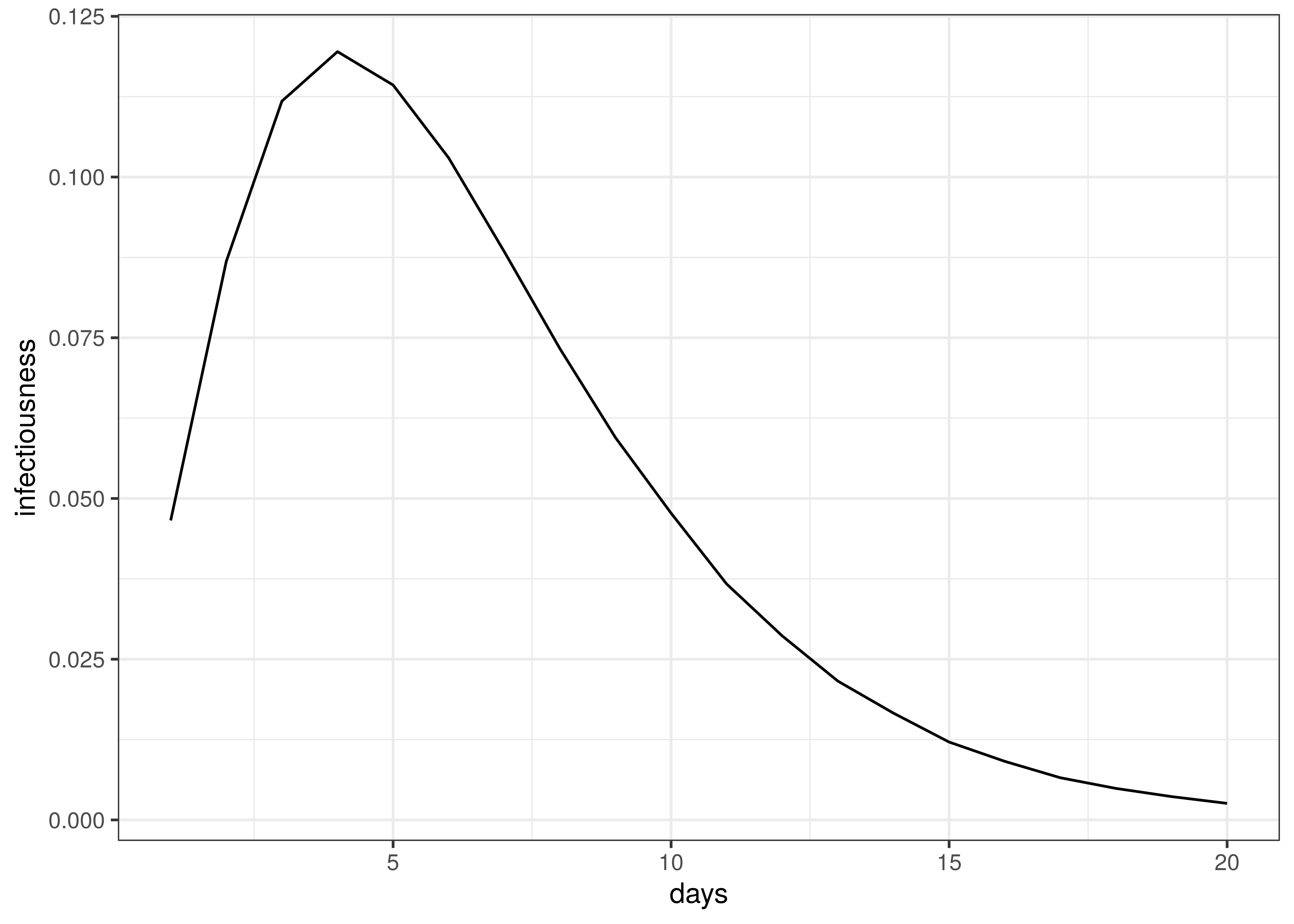
Infectiousness / Serial Interval
Time to death follows this distribution:
\(\pi \sim Gamma(5.1,0.86)+Gamma(17.8,0.45)\)
The distribution of time to death is plotted below.
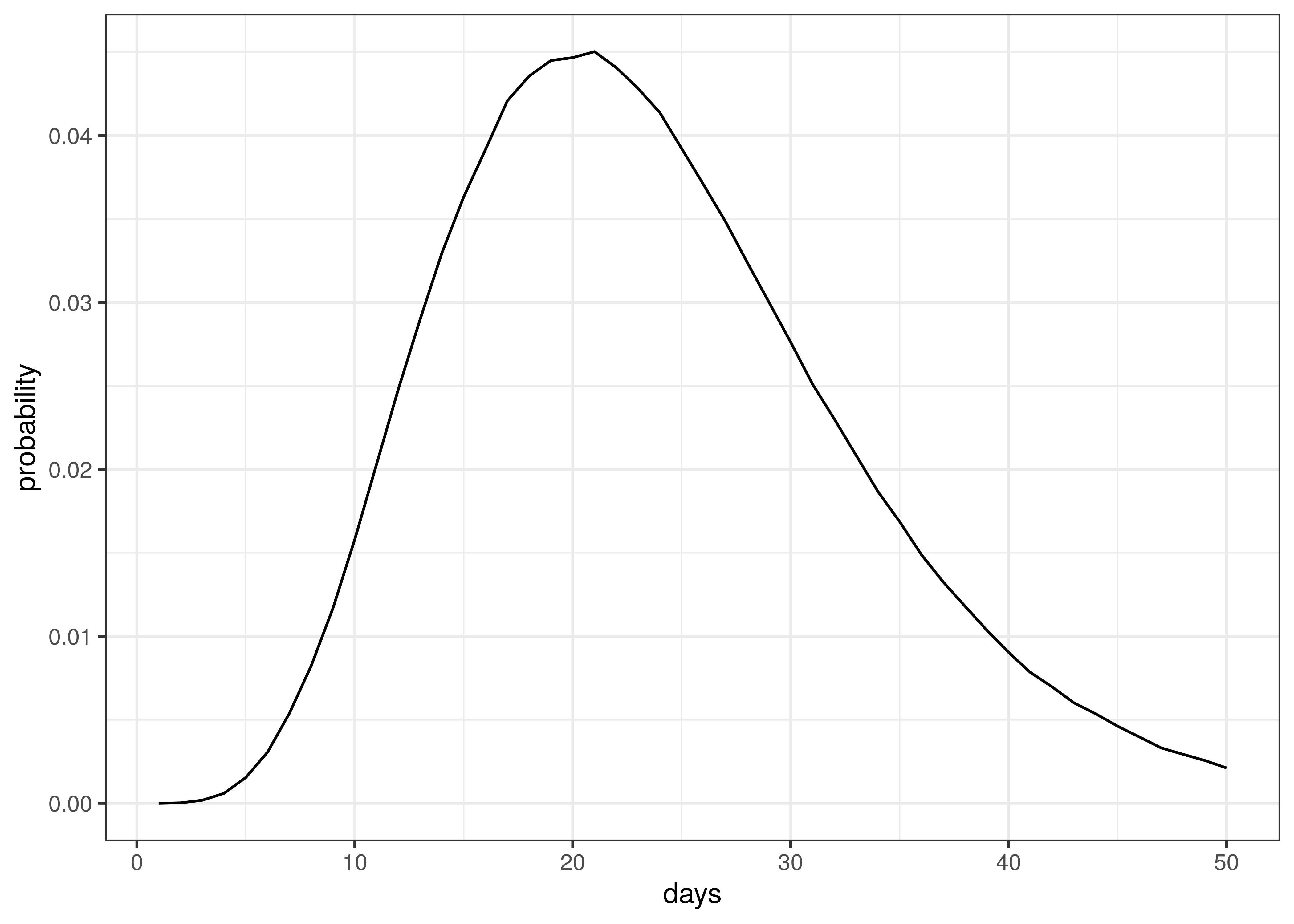
Distribution of Time to Death since Infection
The above implies an average time to death of 23 days.
12.3 Death and Confirmed Case Data
Death and case data were used from [4]. This data set contains provincial case and death data as released by various provinces.
The only adjustments to the data relates to large numbers of deaths reported in Ontario on 2 and 3 October 2020 “due to a data review.” 111 of the deaths reported on these two dates are deaths that occurred during the prior spring and summer (see [19] and [20]). Based on this these deaths were removed from 2 and 3 October and added back in prior days in proportion to deaths reported up un till 30 September 2020. The net effect is no change in reported deaths, but a peak in October is avoided which would have biased calibration of the model.
12.4 Provinces
Provinces are grouped as follows. The province grouping “Territories” are not modelled as there is too few reported deaths to date to model.
| Province | Province Grouping |
|---|---|
| Alberta | Alberta |
| British Columbia | British Columbia |
| Manitoba | Manitoba |
| New Brunswick | Maritime Provinces |
| Newfoundland and Labrador | Maritime Provinces |
| Nova Scotia | Maritime Provinces |
| Nunavut | Territories |
| Northwest Territories | Territories |
| Ontario | Ontario |
| Prince Edward Island | Maritime Provinces |
| Quebec | Quebec |
| Saskatchewan | Saskatchewan |
| Yukon | Territories |
12.5 Infection Fatality Rates (IFR)
This paper uses IFRs per Levin et al. [12]. The IFR (\(ifr_{m}\)) for each province was calculated using the output of the squire R package [21] for Canada. It produces age-specific infection attack rates (IAR). The projection was done using the default parameters for Canada and the resultant attack rate (\(a_{x}\)) for each 5-year age band was obtained (\(x\)).
The IFR formula from [12] was used to calculate an IFR (\(ifr_{x}\) for each age band. For 80+ the age 85 was used. The attack rate and IFR were used together with the per age band IAR and these were applied to provincial populations [22] to calculate an average IFR for each province based on the province’s age profile.
\(ifr_{m}=\frac{\sum_{x}N_{x,m} \cdot a_{x} \cdot ifr_{x} }{\sum_{x}N_{x,m}}\)
Here \(N_{x,m}\) is the population in a particular province (\(m\)) and age band (\(x\)).
Below the resultant \(ifr_{m}\) are tabulated::
| Province | IFR |
|---|---|
| Alberta | 0.73% |
| British Columbia | 1.02% |
| Manitoba | 0.87% |
| Maritime Provinces | 1.11% |
| Ontario | 0.96% |
| Quebec | 1.06% |
| Saskatchewan | 0.89% |
The differences between provinces reflect the different age profiles in those provinces as per [22].
12.6 Mobility Indexes
Google has released aggregated mobility data for various countries and for sub-regions in those countries. These data are generated from devices that have enabled the Location History in Google Maps. This feature is available both on Android and iOS devices but is off by default.
For Canada, these data contain the mobility indexes for each province. These are described in [5] as follows:
- Grocery & pharmacy: Mobility trends for places like grocery markets, food warehouses, farmers markets, specialty food shops, drug stores, and pharmacies.
- Parks: Mobility trends for places like local parks, national parks, public beaches, marinas, dog parks, plazas, and public gardens.
- Transit stations: Mobility trends for places like public transport hubs such as subway, bus, and train stations.
- Retail & recreation: Mobility trends for places like restaurants, cafés, shopping centres, theme parks, museums, libraries, and movie theatres.
- Residential: Mobility trends for places of residence.
- Workplaces: Mobility trends for places of work.
These measure changes in mobility relative to a baseline established before the epidemic. For example, -30% implies a 30% reduction in mobility from pre-COVID-19 mobility.
As per [8] these data were combined into an average mobility index for each province which was an average of all mobility indexes excluding:
- Residential
- Parks
In [1] three indexes were used (Residential, Transit and the rest). This was reduced for this paper due to limited data.
13 Conclusion
This paper has set out to show how a Bayesian model can be fitted to the Canadian data. From the process it becomes clear that there remains significant uncertainty with all matters relating this epidemic. It is therefore likely that the model will not be accurate.
This paper has however attempted to allow for uncertainty using the Bayesian approach here which results in at least some distribution of possible results, some of which are definitely catastrophic and some of which are less severe.
It is hoped that this is a useful contribution to the ongoing research on the epidemic.